Overview of Modeling Approaches for Causal Mediation Analysis

Xiaoni Xu

2026-05-08

This document describes how the six causal mediation analysis approaches including the regression-based approach by Valeri et al. (2013) and VanderWeele et al. (2014), the weighting-based approach by VanderWeele et al. (2014), the inverse odd-ratio weighting approach by Tchetgen Tchetgen (2013), the natural effect model by Vansteelandt et al. (2012), the marginal structural model by VanderWeele et al. (2017), and the $g$-formula approach by Robins (1986) are implemented by the CMAverse package. See publications of these approaches for methodological details.

CMAverse currently supports a single exposure, multiple sequential mediators and a single outcome. When multiple mediators are of interest, CMAverse estimates the joint mediated effect through the set of mediators. CMAverse also supports time varying confounders preceding the mediators.

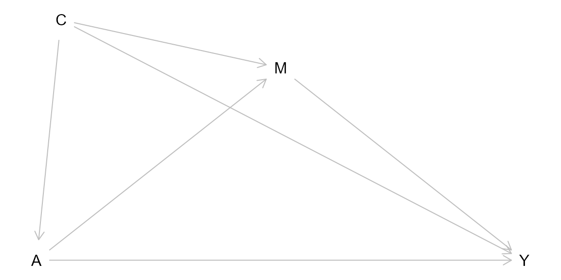
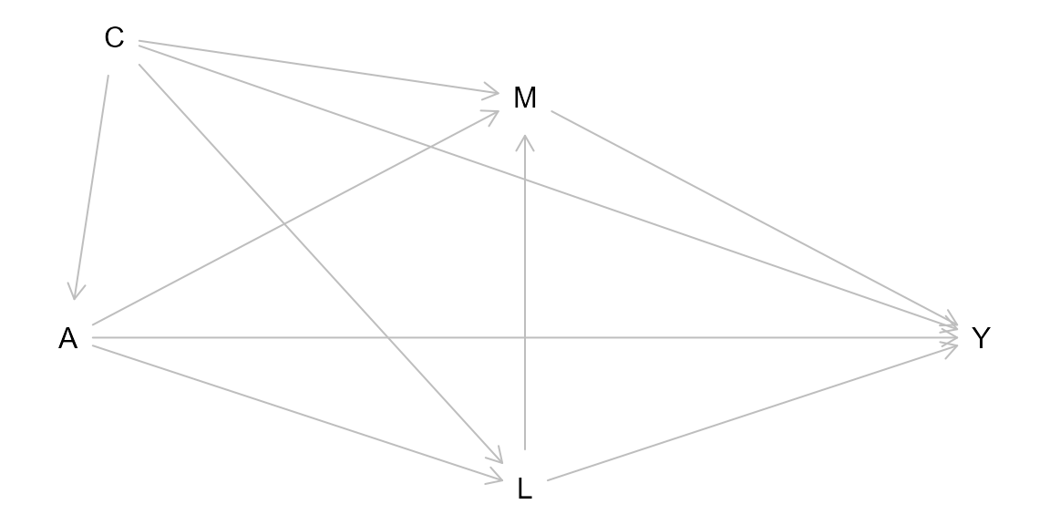
We categorize the causal mediation analysis approaches based on whether the approach can deal with mediator-outcome confounders affected by the exposure. Among the six approaches, only The marginal structural model and the $g$-formula approach are able to deal with mediator-outcome confounders affected by the exposure.

In this document, the outcome and the exposure are denoted as $Y$ and $A$ respectively. The set of exposure-mediator confounders, exposure-outcome confounders and mediator-outcome confounders not affected by the exposure is denoted as $C$. The set of mediators is denoted as $M$ and $M=(M_1,...,M_k)$ follows the temporal order. The set of mediator-outcome confounders affected by the exposure is denoted as $L$ and $L=(L_1,...,L_s)$ follows the temporal order.

Since weights calculated from noncategorical variables are unstable, which hurts the performance of effect estimation and inference, weighted approaches can be implemented only for categorical exposure and mediator(s).

CMAverse Function Parameters

The CMAverse package provides a unified interface for conducting causal mediation analysis through several main functions. Users specify the statistical models and estimation approaches using the following key parameters:

Main Parameters

yreg - Specifies the regression model for the outcome (Y). Options include: - "linear" - Linear regression - "logistic" - Logistic regression for binary outcomes
- "loglinear" - Log-linear regression for count data - "poisson" - Poisson regression for count outcomes - "quasipoisson" - Quasi-Poisson regression - "negbin" - Negative binomial regression - "coxph" - Cox proportional hazards model for survival outcomes - "aft_exp" - Accelerated failure time model with exponential distribution - "aft_weibull" - Accelerated failure time model with Weibull distribution

mreg - Specifies the regression model(s) for the mediator(s) (M). Can be a list for multiple mediators. Options include: - "linear" - Linear regression - "logistic" - Logistic regression for binary mediators - "multinomial" - Multinomial regression for categorical mediators with more than 2 levels

dreg - Specifies the regression model for the confounder model in weighted approaches. Used in inverse probability weighting to estimate treatment weights. Options include: - "linear" - Linear regression - "logistic" - Logistic regression for binary treatment/exposure

ereg - Specifies the regression model for the outcome propensity in certain sensitivity analyses and weighted approaches.

a - The treatment/exposure level of interest (active treatment value)

astar - The reference treatment/exposure level (control value)

m - The value at which to control the mediator (for controlled direct effects)

basecval - A named list specifying baseline confounder values for conditional inference in closed-form parameter function estimation

data - The dataset containing all variables

Additional Common Parameters

nboot - Number of bootstrap samples for confidence interval estimation

CI - Confidence level (e.g., 0.95 for 95% CI)

boot.ci.type - Type of bootstrap confidence intervals (“perc”, “normal”, “basic”, “bca”)

exposure - Name of the exposure/treatment variable

mediators - Name(s) of the mediator variable(s)

outcome - Name of the outcome variable

covariates - Names of baseline confounders (C variables)

postexposure_confounder - Names of post-exposure confounders affected by treatment (L variables)

Function-Specific Parameters

For time-to-event analyses with competing risks: - pathcomprisk() - Implements the mediational g-formula for time-varying mediators and competing risks on the hazard scale - D - List of competing risk/event models
- yreg - The outcome model (typically Aalen or Cox model) - time_points - Time points at which to evaluate mediators - peryr - Person-years divisor for rates - refit - Logical indicating whether to use exact match bootstrapping mode

For causal mediation with multiple mediators: - cmest() - Main function for estimation with multiple sequential mediators - cmsens() - Sensitivity analysis for unmeasured confounding

Users select combinations of these parameters based on their data structure and research question to implement the desired causal mediation analysis approach.

Basic Usage Example

Here is a simple example of conducting causal mediation analysis using CMAverse:

library(CMAverse)

# Example: Regression-based mediation analysis with a continuous outcome
# Suppose we have a dataset 'mydata' with:
# - Exposure: A
# - Mediator: M  
# - Outcome: Y
# - Confounders: C1, C2

# Conduct mediation analysis with linear models
result <- cmest(
  data = mydata,
  model = "rb",                          # regression-based approach
  outcome = "Y",
  exposure = "A",
  mediator = "M",
  basec = c("C1", "C2"),                 # baseline confounders
  yreg = "linear",                       # outcome model: linear regression
  mreg = "linear",                       # mediator model: linear regression
  a = 1,                                 # treatment value (e.g., exposure = 1)
  astar = 0,                             # control value (e.g., exposure = 0)
  mval = 0,                              # mediator value for CDE
  estimation = "paramfunc",              # closed-form parameter functions
  inference = "bootstrap",               # bootstrap for confidence intervals
  nboot = 1000                           # 1000 bootstrap samples
)

# View results
summary(result)

# For time-to-event outcomes with competing risks:
# result <- pathcomprisk(
#   D = list_of_competing_risk_models,
#   mreg = list_of_mediator_models,
#   mvar = c("M1", "M2"),
#   yreg = aalen_cox_model,
#   avar = "A",
#   a = 1,
#   astar = 0,
#   data = mydata,
#   nboot = 1000
# )

No Confounders Affected by the Exposure

DAG

Estimands

For a continuous outcome, causal effects are estimated on the difference scale (summarized in table 1). For a categorical, count, or survival outcome, causal effects are estimated on the ratio scale (summarized in table 2). See Valeri et al. (2013) and VanderWeele (2015) for details about these effects.

Table 1: Causal Effects on the Difference Scale

Full Name	Abbreviation	Formula
Controlled Direct Effect	$CDE$	$E[Y_{am}-Y_{a^*m}]$
Pure Natural Direct Effect	$PNDE$	$E[Y_{aM_a^*}-Y_{a^*M_a^*}]$
Total Natural Direct Effect	$TNDE$	$E[Y_{aM_a}-Y_{a^*M_a}]$
Pure Natural Indirect Effect	$PNIE$	$E[Y_{a^*M_a}-Y_{a^*M_a^*}]$
Total Natural Indirect Effect	$TNIE$	$E[Y_{aM_a}-Y_{aM_a^*}]$
Total Effect	$TE$	$PNDE+TNIE$ or $TNDE+PNIE$
Reference Interaction	$INT_{ref}$	$PNDE-CDE$
Mediated Interaction	$INT_{med}$	$TNIE-PNIE$
Proportion $CDE$	$prop^{CDE}$	$CDE/TE$
Proportion $INT_{ref}$	$prop^{INT_{ref}}$	$INT_{ref}/TE$
Proportion $INT_{med}$	$prop^{INT_{med}}$	$INT_{med}/TE$
Proportion $PNIE$	$prop^{PNIE}$	$PNIE/TE$
Proportion Mediated	$PM$	$TNIE/TE$
Proportion Attributable to Interaction	$INT$	$(INT_{ref}+INT_{med})/TE$
Proportion Eliminated	$PE$	$(INT_{ref}+INT_{med}+PNIE)/TE$
Residual Disparity	$RD$	$P(S_g>s|A=a,C) - P(S_g>s|A=a^*,C)$
Shifting Distribution Effect	$SD$	$P(S_{g'}>s|A=a,C) - P(S_g>s|A=a,C)$
Note:
$a$ and $a^*$ are the active and control values for $A$ respectively. $m$ is the value at which $M$ is controlled. $M_a$ denotes the counterfactual value of $M$ that would have been observed had $A$ been set to be $a$. $Y_{am}$ denotes the counterfactual value of $Y$ that would have been observed had $A$ been set to be $a$, and $M$ to be $m$. $Y_{aMa*}$ denotes the counterfactual value of $Y$ that would have been observed had $A$ been set to be $a$, and $M$ to be the counterfactual value $M_{a*}$.

Table 2: Causal Effects on the Ratio Scale

Full Name	Abbreviation	Formula
Controlled Direct Effect	$R^{CDE}$	$E[Y_{am}]/E[Y_{a^*m}]$
Pure Natural Direct Effect	$R^{PNDE}$	$E[Y_{aM_a^*}]/E[Y_{a^*M_a^*}]$
Total Natural Direct Effect	$R^{TNDE}$	$E[Y_{aM_a}]/E[Y_{a^*M_a}]$
Pure Natural Indirect Effect	$R^{PNIE}$	$E[Y_{a^*M_a}]/E[Y_{a^*M_a^*}]$
Total Natural Indirect Effect	$R^{TNIE}$	$E[Y_{aM_a}]/E[Y_{aM_a^*}]$
Total Effect	$R^{TE}$	$R^{PNDE}\times R^{TNIE}$ or $R^{TNDE}\times R^{PNIE}$
Excess Ratio due to Controlled Direct Effect	$ER^{CDE}$	$(E[Y_{am}-Y_{a^*m}])/E[Y_{a^*M_a^*}]$
Excess Ratio due to Reference Interaction	$ER^{INT_{ref}}$	$R^{PNDE}-1-ER^{CDE}$
Excess Ratio due to Mediated Interaction	$ER^{INT_{med}}$	$R^{TNIE}*R^{PNDE}-R^{PNDE}-R^{PNIE}+1$
Excess Ratio due to Pure Natural Indirect Effect	$ER^{PNIE}$	$R^{PNIE}-1$
Proportion $ER^{CDE}$	$prop^{ER^{CDE}}$	$ER^{CDE}/(R^{TE}-1)$
Proportion $ER^{INT_{ref}}$	$prop^{ER^{INT_{ref}}}$	$ER^{INT_{ref}}/(R^{TE}-1)$
Proportion $ER^{INT_{med}}$	$prop^{ER^{INT_{med}}}$	$ER^{INT_{med}}/(R^{TE}-1)$
Proportion $ER^{PNIE}$	$prop^{ER^{PNIE}}$	$ER^{PNIE}/(R^{TE}-1)$
Proportion Mediated	$PM$	$(R^{PNDE}*(R^{TNIE}-1))/(R^{TE}-1)$
Proportion Attributable to Interaction	$INT$	$(ER^{INT_{ref}}+ER^{INT_{med}})/(R^{TE}-1)$
Proportion Eliminated	$PE$	$(ER^{INT_{ref}}+ER^{INT_{med}}+ER^{PNIE})/(R^{TE}-1)$
Note:
$a$ and $a^*$ are the active and control values for $A$ respectively. $m$ is the value at which $M$ is controlled. $M_a$ denotes the counterfactual value of $M$ that would have been observed had $A$ been set to be $a$. $Y_{am}$ denotes the counterfactual value of $Y$ that would have been observed had $A$ been set to be $a$, and $M$ to be $m$. $Y_{aMa*}$ denotes the counterfactual value of $Y$ that would have been observed had $A$ been set to be $a$, and $M$ to be the counterfactual value $M_{a*}$. If $Y$ is categorical, $E[Y]$ represents the probability of $Y=y$ where $y$ is a pre-specified value of $Y$.

The Regression-based Approach

With the regression-based approach, all causal effects are estimated through either closed-form parameter function estimation or direct counterfactual imputation estimation. Standard errors of causal effects are estimated through either the delta method or bootstrapping.

Closed-form Parameter Function Estimation

Closed-form parameter function estimation is available when there is only a single mediator, i.e., $M=M_1$. Also, yreg must be chosen from linear, logistic, loglinear, poisson, quasipoisson, negbin, coxph, aft_exp and aft_weibull. mreg must be chosen from linear, logistic and multinomial. To use yreg = "logistic" and yreg = "coxph" in closed-form parameter function estimation, the outcome must be rare. Additionally, the causal effects estimated through closed-form parameter function estimation are conditional on the value of $C$ specified by the basecval argument. Closed-form parameter functions are summarized below.

Linear yreg, Linear mreg and Noncategorical Exposure

If the exposure is not categorical, yreg="linear" and mreg=list("linear"), CMAverse estimates the causal effects by the following steps:

1. Fit a linear regression model for the mediator: $$E[M|A,C]=\beta_0+\beta_1A+\beta_2'C$$

2. Fit a linear regression model for the outcome: $$E[Y|A,M,C]=\theta_0+\theta_1A+\theta_2M+\theta_3AM+\theta_4'C$$

3. Estimate $CDE$, $PNDE$, $TNDE$, $PNIE$ and $TNIE$ by the following parameter functions:

   • $CDE=(\theta_1+\theta_3m)(a-a^*)$
   • $PNDE=\{\theta_1+\theta_3(\beta_0+\beta_1a^*+\beta_2'c)\}(a-a^*)$
   • $TNDE=\{\theta_1+\theta_3(\beta_0+\beta_1a+\beta_2'c)\}(a-a^*)$
   • $PNIE=(\theta_2\beta_1+\theta_3\beta_1a^*)(a-a^*)$
   • $TNIE=(\theta_2\beta_1+\theta_3\beta_1a)(a-a^*)$

4. Calculate other effects using formulas in table 1.

Linear yreg, Linear mreg and Categorical Exposure

If the exposure is categorical, yreg="linear" and mreg=list("linear"), CMAverse estimates the causal effects by the following steps:

1. Fit a linear regression model for the mediator: $$E[M|A,C]=\beta_0+\sum_{h=1}^H\beta_{1h}I\{A=h\}+\beta_2'C$$

2. Fit a linear regression model for the outcome: $$E[Y|A,M,C]=\theta_0+\sum_{h=1}^H\theta_{1h}I\{A=h\}+\theta_2M+\sum_{h=1}^H\theta_{3h}I\{A=h\}M+\theta_4'C$$

3. Estimate $CDE$, $PNDE$, $TNDE$, $PNIE$ and $TNIE$ by the following parameter functions:

   • $CDE=\sum_{h=1}^H\theta_{1h}I\{a=h\}-\sum_{h=1}^H\theta_{1h}I\{a^*=h\}+(\sum_{h=1}^H\theta_{3h}I\{a=h\}-\sum_{h=1}^H\theta_{3h}I\{a^*=h\})m$
   • $PNDE=\sum_{h=1}^H\theta_{1h}I\{a=h\}-\sum_{h=1}^H\theta_{1h}I\{a^*=h\}+(\sum_{h=1}^H\theta_{3h}I\{a=h\}-\sum_{h=1}^H\theta_{3h}I\{a^*=h\})(\beta_0+\sum_{h=1}^H\beta_{1h}I\{a^*=h\}+\beta_2'c)$
   • $TNDE=\sum_{h=1}^H\theta_{1h}I\{a=h\}-\sum_{h=1}^H\theta_{1h}I\{a^*=h\}+(\sum_{h=1}^H\theta_{3h}I\{a=h\}-\sum_{h=1}^H\theta_{3h}I\{a^*=h\})(\beta_0+\sum_{h=1}^H\beta_{1h}I\{a=h\}+\beta_2'c)$
   • $PNIE=(\theta_2+\sum_{h=1}^H\theta_{3h}I\{a^*=h\})(\sum_{h=1}^H\beta_{1h}I\{a=h\}-\sum_{h=1}^H\beta_{1h}I\{a^*=h\})$
   • $TNIE=(\theta_2+\sum_{h=1}^H\theta_{3h}I\{a=h\})(\sum_{h=1}^H\beta_{1h}I\{a=h\}-\sum_{h=1}^H\beta_{1h}I\{a^*=h\})$

4. Calculate other effects using formulas in table 1.

Linear yreg, Logistic mreg and Noncategorical Exposure

If the exposure is not categorical, yreg="linear" and mreg=list("logistic"), CMAverse estimates the causal effects by the following steps:

1. Fit a logistic regression model for the mediator: $$logitE[M|A,C]=\beta_0+\beta_1A+\beta_2'C$$

2. Fit a linear regression model for the outcome: $$E[Y|A,M,C]=\theta_0+\theta_1A+\theta_2M+\theta_3AM+\theta_4'C$$

3. Estimate $CDE$, $PNDE$, $TNDE$, $PNIE$ and $TNIE$ by the following parameter functions:

   • $CDE=(\theta_1+\theta_3m)(a-a^*)$
   • $PNDE=\{\theta_1+\theta_3\frac{exp(\beta_0+\beta_1a^*+\beta_2'c)}{1+exp(\beta_0+\beta_1a^*+\beta_2'c)}\}(a-a^*)$
   • $TNDE=\{\theta_1+\theta_3\frac{exp(\beta_0+\beta_1a+\beta_2'c)}{1+exp(\beta_0+\beta_1a+\beta_2'c)}\}(a-a^*)$
   • $PNIE=(\theta_2+\theta_3a^*)(\frac{exp(\beta_0+\beta_1a+\beta_2'c)}{1+exp(\beta_0+\beta_1a+\beta_2'c)}-\frac{exp(\beta_0+\beta_1a^*+\beta_2'c)}{1+exp(\beta_0+\beta_1a^*+\beta_2'c)})$
   • $TNIE=(\theta_2+\theta_3a)(\frac{exp(\beta_0+\beta_1a+\beta_2'c)}{1+exp(\beta_0+\beta_1a+\beta_2'c)}-\frac{exp(\beta_0+\beta_1a^*+\beta_2'c)}{1+exp(\beta_0+\beta_1a^*+\beta_2'c)})$

4. Calculate other effects using formulas in table 1.

Linear yreg, Logistic mreg and Categorical Exposure

If the exposure is categorical, yreg="linear" and mreg=list("logistic"), CMAverse estimates the causal effects by the following steps:

1. Fit a logistic regression model for the mediator: $$logitE[M|A,C]=\beta_0+\sum_{h=1}^H\beta_{1h}I\{A=h\}+\beta_2'C$$

2. Fit a linear regression model for the outcome: $$E[Y|A,M,C]=\theta_0+\sum_{h=1}^H\theta_{1h}I\{A=h\}+\theta_2M+\sum_{h=1}^H\theta_{3h}I\{A=h\}M+\theta_4'C$$

3. Estimate $CDE$, $PNDE$, $TNDE$, $PNIE$ and $TNIE$ by the following parameter functions:

   • $CDE=\sum_{h=1}^H\theta_{1h}I\{a=h\}-\sum_{h=1}^H\theta_{1h}I\{a^*=h\}+(\sum_{h=1}^H\theta_{3h}I\{a=h\}-\sum_{h=1}^H\theta_{3h}I\{a^*=h\})m$
   • $PNDE=\sum_{h=1}^H\theta_{1h}I\{a=h\}-\sum_{h=1}^H\theta_{1h}I\{a^*=h\}+(\sum_{h=1}^H\theta_{3h}I\{a=h\}-\sum_{h=1}^H\theta_{3h}I\{a^*=h\})\frac{exp(\beta_0+\sum_{h=1}^H\beta_{1h}I\{a^*=h\}+\beta_2'c)}{1+exp(\beta_0+\sum_{h=1}^H\beta_{1h}I\{a^*=h\}+\beta_2'c)}$
   • $TNDE=\sum_{h=1}^H\theta_{1h}I\{a=h\}-\sum_{h=1}^H\theta_{1h}I\{a^*=h\}+(\sum_{h=1}^H\theta_{3h}I\{a=h\}-\sum_{h=1}^H\theta_{3h}I\{a^*=h\})\frac{exp(\beta_0+\sum_{h=1}^H\beta_{1h}I\{a=h\}+\beta_2'c)}{1+exp(\beta_0+\sum_{h=1}^H\beta_{1h}I\{a=h\}+\beta_2'c)}$
   • $PNIE=(\theta_2+\sum_{h=1}^H\theta_{3h}I\{a^*=h\})(\frac{exp(\beta_0+\sum_{h=1}^H\beta_{1h}I\{a=h\}+\beta_2'c)}{1+exp(\beta_0+\sum_{h=1}^H\beta_{1h}I\{a=h\}+\beta_2'c)}-\frac{exp(\beta_0+\sum_{h=1}^H\beta_{1h}I\{a^*=h\}+\beta_2'c)}{1+exp(\beta_0+\sum_{h=1}^H\beta_{1h}I\{a^*=h\}+\beta_2'c)})$
   • $TNIE=(\theta_2+\sum_{h=1}^H\theta_{3h}I\{a=h\})(\frac{exp(\beta_0+\sum_{h=1}^H\beta_{1h}I\{a=h\}+\beta_2'c)}{1+exp(\beta_0+\sum_{h=1}^H\beta_{1h}I\{a=h\}+\beta_2'c)}-\frac{exp(\beta_0+\sum_{h=1}^H\beta_{1h}I\{a^*=h\}+\beta_2'c)}{1+exp(\beta_0+\sum_{h=1}^H\beta_{1h}I\{a^*=h\}+\beta_2'c)})$

4. Calculate other effects using formulas in table 1.

Linear yreg, Multinomial mreg and Noncategorical Exposure

If the exposure is not categorical, yreg="linear" and mreg=list("multinomial"), CMAverse estimates the causal effects by the following steps:

1. Fit a multinomial regression model for the mediator: $$log\frac{E[M=j|A,C]}{E[M=0|A,C]}=\beta_{0j}+\beta_{1j}A+\beta_{2j}'C, j=1,2,...,J$$

2. Fit a linear regression model for the outcome: $$E[Y|A,M,C]=\theta_0+\theta_1A+\sum_{j=1}^J\theta_{2j}I\{M=j\}+A\sum_{j=1}^J\theta_{3j}I\{M=j\}+\theta_4'C$$

3. Estimate $CDE$, $PNDE$, $TNDE$, $PNIE$ and $TNIE$ by the following parameter functions:

   • $CDE=(\theta_1+\sum_{j=1}^J\theta_{3j}I\{m=j\})(a-a^*)$
   • $PNDE=\{\theta_1+\frac{\sum_{j=1}^J\theta_{3j}exp(\beta_{0j}+\beta_{1j}a^*+\beta_{2j}'c)}{1+\sum_{j=1}^Jexp(\beta_{0j}+\beta_{1j}a^*+\beta_{2j}'c)}\}(a-a^*)$
   • $TNDE=\{\theta_1+\frac{\sum_{j=1}^J\theta_{3j}exp(\beta_{0j}+\beta_{1j}a+\beta_{2j}'c)}{1+\sum_{j=1}^Jexp(\beta_{0j}+\beta_{1j}a+\beta_{2j}'c)}\}(a-a^*)$
   • $PNIE=\frac{\sum_{j=1}^J(\theta_{2j}+\theta_{3j}a^*)exp(\beta_{0j}+\beta_{1j}a+\beta_{2j}'c)}{1+\sum_{j=1}^Jexp(\beta_{0j}+\beta_{1j}a+\beta_{2j}'c)}-\frac{\sum_{j=1}^J(\theta_{2j}+\theta_{3j}a^*)exp(\beta_{0j}+\beta_{1j}a^*+\beta_{2j}'c)}{1+\sum_{j=1}^Jexp(\beta_{0j}+\beta_{1j}a^*+\beta_{2j}'c)}$
   • $TNIE=\frac{\sum_{j=1}^J(\theta_{2j}+\theta_{3j}a)exp(\beta_{0j}+\beta_{1j}a+\beta_{2j}'c)}{1+\sum_{j=1}^Jexp(\beta_{0j}+\beta_{1j}a+\beta_{2j}'c)}-\frac{\sum_{j=1}^J(\theta_{2j}+\theta_{3j}a)exp(\beta_{0j}+\beta_{1j}a^*+\beta_{2j}'c)}{1+\sum_{j=1}^Jexp(\beta_{0j}+\beta_{1j}a^*+\beta_{2j}'c)}$

4. Calculate other effects using formulas in table 1.

Linear yreg, Multinomial mreg and Categorical Exposure

If the exposure is categorical, yreg="linear" and mreg=list("multinomial"), CMAverse estimates the causal effects by the following steps:

1. Fit a multinomial regression model for the mediator: $$log\frac{E[M=j|A,C]}{E[M=0|A,C]}=\beta_{0j}+\sum_{h=1}^H\beta_{1jh}I\{A=h\}+\beta_{2j}'C, j=1,2,...,J$$

2. Fit a linear regression model for the outcome: $$E[Y|A,M,C]=\theta_0+\sum_{h=1}^H\theta_{1h}I\{A=h\}+\sum_{j=1}^J\theta_{2j}I\{M=j\}+\sum_{j=1}^J\sum_{h=1}^H\theta_{3jh}I\{M=j\}I\{A=h\}+\theta_4'C$$

3. Estimate $CDE$, $PNDE$, $TNDE$, $PNIE$ and $TNIE$ by the following parameter functions:

   • $CDE=\sum_{h=1}^H\theta_{1h}I\{a=h\}-\sum_{h=1}^H\theta_{1h}I\{a^*=h\}+(\sum_{j=1}^J\sum_{h=1}^H\theta_{3jh}I\{m=j\}I\{a=h\}-\sum_{j=1}^J\sum_{h=1}^H\theta_{3jh}I\{m=j\}I\{a^*=h\})$
   • $PNDE=\sum_{h=1}^H\theta_{1h}I\{a=h\}-\sum_{h=1}^H\theta_{1h}I\{a^*=h\}+\frac{\sum_{j=1}^J(\sum_{h=1}^H\theta_{3jh}I\{a=h\}-\sum_{h=1}^H\theta_{3jh}I\{a^*=h\})exp(\beta_{0j}+\sum_{h=1}^H\beta_{1jh}I\{a^*=h\}+\beta_{2j}'c)}{1+\sum_{j=1}^Jexp(\beta_{0j}+\sum_{h=1}^H\beta_{1jh}I\{a^*=h\}+\beta_{2j}'c)}$
   • $TNDE=\sum_{h=1}^H\theta_{1h}I\{a=h\}-\sum_{h=1}^H\theta_{1h}I\{a^*=h\}+\frac{\sum_{j=1}^J(\sum_{h=1}^H\theta_{3jh}I\{a=h\}-\sum_{h=1}^H\theta_{3jh}I\{a^*=h\})exp(\beta_{0j}+\sum_{h=1}^H\beta_{1jh}I\{a=h\}+\beta_{2j}'c)}{1+\sum_{j=1}^Jexp(\beta_{0j}+\sum_{h=1}^H\beta_{1jh}I\{a=h\}+\beta_{2j}'c)}$
   • $PNIE=\frac{\sum_{j=1}^J(\theta_{2j}+\sum_{h=1}^H\theta_{3jh}I\{a^*=h\})exp(\beta_{0j}+\sum_{h=1}^H\beta_{1jh}I\{a=h\}+\beta_{2j}'c)}{1+\sum_{j=1}^Jexp(\beta_{0j}+\sum_{h=1}^H\beta_{1jh}I\{a=h\}+\beta_{2j}'c)}-\frac{\sum_{j=1}^J(\theta_{2j}+\sum_{h=1}^H\theta_{3jh}I\{a^*=h\})exp(\beta_{0j}+\sum_{h=1}^H\beta_{1jh}I\{a^*=h\}+\beta_{2j}'c)}{1+\sum_{j=1}^Jexp(\beta_{0j}+\sum_{h=1}^H\beta_{1jh}I\{a^*=h\}+\beta_{2j}'c)}$
   • $TNIE=\frac{\sum_{j=1}^J(\theta_{2j}+\sum_{h=1}^H\theta_{3jh}I\{a=h\})exp(\beta_{0j}+\sum_{h=1}^H\beta_{1jh}I\{a=h\}+\beta_{2j}'c)}{1+\sum_{j=1}^Jexp(\beta_{0j}+\sum_{h=1}^H\beta_{1jh}I\{a=h\}+\beta_{2j}'c)}-\frac{\sum_{j=1}^J(\theta_{2j}+\sum_{h=1}^H\theta_{3jh}I\{a=h\})exp(\beta_{0j}+\sum_{h=1}^H\beta_{1jh}I\{a^*=h\}+\beta_{2j}'c)}{1+\sum_{j=1}^Jexp(\beta_{0j}+\sum_{h=1}^H\beta_{1jh}I\{a^*=h\}+\beta_{2j}'c)}$

4. Calculate other effects using formulas in table 1.

Nonlinear yreg, Linear mreg and Noncategorical Exposure

If the exposure is not categorical, yreg!="linear" and mreg=list("linear"), CMAverse estimates the causal effects by the following steps:

1. Fit a linear regression model for the mediator: $$E[M|A,C]=\beta_0+\beta_1A+\beta_2'C+\epsilon_M,\epsilon_M\sim N(0,\sigma^2)$$

2. Fit the specified regression model for the outcome: $$g(E[Y|A,M,C])=\theta_0+\theta_1A+\theta_2M+\theta_3AM+\theta_4'C$$

3. Estimate $R^{CDE}$, $R^{PNDE}$, $R^{TNDE}$, $R^{PNIE}$, $R^{TNIE}$ and $ER^{CDE}$ by the following parameter functions:

   • $R^{CDE}=exp((\theta_1+\theta_3m)(a-a^*))$
   • $R^{PNDE}=exp(\{\theta_1+\theta_3(\beta_0+\beta_1a^*+\beta_2'c+\theta_2\sigma^2)\}(a-a^*)+0.5\theta_3^2\sigma^2(a^2-a^{*2}))$
   • $R^{TNDE}=exp(\{\theta_1+\theta_3(\beta_0+\beta_1a+\beta_2'c+\theta_2\sigma^2)\}(a-a^*)+0.5\theta_3^2\sigma^2(a^2-a^{*2}))$
   • $R^{PNIE}=exp((\theta_2\beta_1+\theta_3\beta_1a^*)(a-a^*))$
   • $R^{TNIE}=exp((\theta_2\beta_1+\theta_3\beta_1a)(a-a^*))$
   • $ER^{CDE}=(exp(\theta_1(a-a^*)+\theta_3am)-exp(\theta_3a^*m))exp(\theta_2m-(\theta_2+\theta_3a^*)(\beta_0+\beta_1a^*+\beta_2'c)-0.5(\theta_2+\theta_3a^*)^2\sigma^2)$

4. Calculate other effects using formulas in table 2.

Nonlinear yreg, Linear mreg and Categorical Exposure

If the exposure is categorical, yreg!="linear" and mreg=list("linear"), CMAverse estimates the causal effects by the following steps:

1. Fit a linear regression model for the mediator: $$E[M|A,C]=\beta_0+\sum_{h=1}^H\beta_{1h}I\{A=h\}+\beta_2'C+\epsilon_M,\epsilon_M\sim N(0,\sigma^2)$$

2. Fit the specified regression model for the outcome: $$g(E[Y|A,M,C])=\theta_0+\sum_{h=1}^H\theta_{1h}I\{A=h\}+\theta_2M+\sum_{h=1}^H\theta_{3h}I\{A=h\}M+\theta_4'C$$

3. Estimate $R^{CDE}$, $R^{PNDE}$, $R^{TNDE}$, $R^{PNIE}$, $R^{TNIE}$ and $ER^{CDE}$ by the following parameter functions:

   • $R^{CDE}=exp(\sum_{h=1}^H\theta_{1h}I\{a=h\}-\sum_{h=1}^H\theta_{1h}I\{a^*=h\}+(\sum_{h=1}^H\theta_{3h}I\{a=h\}-\sum_{h=1}^H\theta_{3h}I\{a^*=h\})m)$
   • $R^{PNDE}=exp(\sum_{h=1}^H\theta_{1h}I\{a=h\}-\sum_{h=1}^H\theta_{1h}I\{a^*=h\}+(\sum_{h=1}^H\theta_{3h}I\{a=h\}-\sum_{h=1}^H\theta_{3h}I\{a^*=h\})(\beta_0+\sum_{h=1}^H\beta_{1h}I\{a^*=h\}+\beta_2'c+\theta_2\sigma^2)+0.5\sigma^2(\sum_{h=1}^H\theta_{3h}^2I\{a=h\}-\sum_{h=1}^H\theta_{3h}^2I\{a^*=h\}))$
   • $R^{TNDE}=exp(\sum_{h=1}^H\theta_{1h}I\{a=h\}-\sum_{h=1}^H\theta_{1h}I\{a^*=h\}+(\sum_{h=1}^H\theta_{3h}I\{a=h\}-\sum_{h=1}^H\theta_{3h}I\{a^*=h\})(\beta_0+\sum_{h=1}^H\beta_{1h}I\{a=h\}+\beta_2'c+\theta_2\sigma^2)+0.5\sigma^2(\sum_{h=1}^H\theta_{3h}^2I\{a=h\}-\sum_{h=1}^H\theta_{3h}^2I\{a^*=h\}))$
   • $R^{PNIE}=exp(\theta_2(\sum_{h=1}^H\beta_{1h}I\{a=h\}-\sum_{h=1}^H\beta_{1h}I\{a^*=h\})+\sum_{h=1}^H\theta_{3h}I\{a^*=h\}(\sum_{h=1}^H\beta_{1h}I\{a=h\}-\sum_{h=1}^H\beta_{1h}I\{a^*=h\}))$
   • $R^{TNIE}=exp(\theta_2(\sum_{h=1}^H\beta_{1h}I\{a=h\}-\sum_{h=1}^H\beta_{1h}I\{a^*=h\})+\sum_{h=1}^H\theta_{3h}I\{a=h\}(\sum_{h=1}^H\beta_{1h}I\{a=h\}-\sum_{h=1}^H\beta_{1h}I\{a^*=h\}))$
   • $ER^{CDE}=(exp(\sum_{h=1}^H\theta_{1h}I\{a=h\}-\sum_{h=1}^H\theta_{1h}I\{a^*=h\}+\sum_{h=1}^H\theta_{3h}I\{a=h\}m)-exp(\sum_{h=1}^H\theta_{3h}I\{a^*=h\}m))exp(\theta_2m-(\theta_2+\sum_{h=1}^H\theta_{3h}I\{a^*=h\})(\beta_0+\sum_{h=1}^H\beta_{1h}I\{a^*=h\}+\beta_2'c)-0.5(\theta_2+\sum_{h=1}^H\theta_{3h}I\{a^*=h\})^2\sigma^2)$

4. Calculate other effects using formulas in table 2.

Nonlinear yreg, Logistic mreg and Noncategorical Exposure

If the exposure is not categorical, yreg!="linear" and mreg=list("logistic"), CMAverse estimates the causal effects by the following steps:

1. Fit a logistic regression model for the mediator: $$logitE[M|A,C]=\beta_0+\beta_1A+\beta_2'C$$

2. Fit the specified regression model for the outcome: $$g(E[Y|A,M,C])=\theta_0+\theta_1A+\theta_2M+\theta_3AM+\theta_4'C$$

3. Estimate $R^{CDE}$, $R^{PNDE}$, $R^{TNDE}$, $R^{PNIE}$, $R^{TNIE}$ and $ER^{CDE}$ by the following parameter functions:

   • $R^{CDE}=exp((\theta_1+\theta_3m)(a-a^*))$
   • $R^{PNDE}=\frac{exp(\theta_1a)\{1+exp(\theta_2+\theta_3a+\beta_0+\beta_1a^*+\beta_2'c)\}}{exp(\theta_1a^*)\{1+exp(\theta_2+\theta_3a^*+\beta_0+\beta_1a^*+\beta_2'c)\}}$
   • $R^{TNDE}=\frac{exp(\theta_1a)\{1+exp(\theta_2+\theta_3a+\beta_0+\beta_1a+\beta_2'c)\}}{exp(\theta_1a^*)\{1+exp(\theta_2+\theta_3a^*+\beta_0+\beta_1a+\beta_2'c)\}}$
   • $R^{PNIE}=\frac{\{1+exp(\beta_0+\beta_1a^*+\beta_2'c)\}\{1+exp(\theta_2+\theta_3a^*+\beta_0+\beta_1a+\beta_2'c)\}}{\{1+exp(\beta_0+\beta_1a+\beta_2'c)\}\{1+exp(\theta_2+\theta_3a^*+\beta_0+\beta_1a^*+\beta_2'c)\}}$
   • $R^{TNIE}=\frac{\{1+exp(\beta_0+\beta_1a^*+\beta_2'c)\}\{1+exp(\theta_2+\theta_3a+\beta_0+\beta_1a+\beta_2'c)\}}{\{1+exp(\beta_0+\beta_1a+\beta_2'c)\}\{1+exp(\theta_2+\theta_3a+\beta_0+\beta_1a^*+\beta_2'c)\}}$
   • $ER^{CDE}=\frac{exp(\theta_2m)(exp(\theta_1(a-a^*)+\theta_3am)-exp(\theta_3a^*m))(1+exp(\beta_0+\beta_1a^*+\beta_2'c))}{1+exp(\beta_0+\beta_1a^*+\beta_2'c+\theta_2+\theta_3a^*)}$

4. Calculate other effects using formulas in table 2.

Nonlinear yreg, Logistic mreg and Categorical Exposure

If the exposure is categorical, yreg!="linear" and mreg=list("logistic"), CMAverse estimates the causal effects by the following steps:

1. Fit a logistic regression model for the mediator: $$logitE[M|A,C]=\beta_0+\sum_{h=1}^H\beta_{1h}I\{A=h\}+\beta_2'C$$

2. Fit the specified regression model for the outcome: $$g(E[Y|A,M,C])=\theta_0+\sum_{h=1}^H\theta_{1h}I\{A=h\}+\theta_2M+\sum_{h=1}^H\theta_{3h}I\{A=h\}M+\theta_4'C$$

3. Estimate $R^{CDE}$, $R^{PNDE}$, $R^{TNDE}$, $R^{PNIE}$, $R^{TNIE}$ and $ER^{CDE}$ by the following parameter functions:

   • $R^{CDE}=exp(\sum_{h=1}^H\theta_{1h}I\{a=h\}-\sum_{h=1}^H\theta_{1h}I\{a^*=h\}+(\sum_{h=1}^H\theta_{3h}I\{a=h\}-\sum_{h=1}^H\theta_{3h}I\{a^*=h\})m)$
   • $R^{PNDE}=\frac{exp(\sum_{h=1}^H\theta_{1h}I\{a=h\})\{1+exp(\theta_2+\sum_{h=1}^H\theta_{3h}I\{a=h\}+\beta_0+\sum_{h=1}^H\beta_{1h}I\{a^*=h\}+\beta_2'c)\}}{exp(\sum_{h=1}^H\theta_{1h}I\{a^*=h\})\{1+exp(\theta_2+\sum_{h=1}^H\theta_{3h}I\{a^*=h\}+\beta_0+\sum_{h=1}^H\beta_{1h}I\{a^*=h\}+\beta_2'c)\}}$
   • $R^{TNDE}=\frac{exp(\sum_{h=1}^H\theta_{1h}I\{a=h\})\{1+exp(\theta_2+\sum_{h=1}^H\theta_{3h}I\{a=h\}+\beta_0+\sum_{h=1}^H\beta_{1h}I\{a=h\}+\beta_2'c)\}}{exp(\sum_{h=1}^H\theta_{1h}I\{a^*=h\})\{1+exp(\theta_2+\sum_{h=1}^H\theta_{3h}I\{a^*=h\}+\beta_0+\sum_{h=1}^H\beta_{1h}I\{a=h\}+\beta_2'c)\}}$
   • $R^{PNIE}=\frac{\{1+exp(\beta_0+\sum_{h=1}^H\beta_{1h}I\{a^*=h\}+\beta_2'c)\}\{1+exp(\theta_2+\sum_{h=1}^H\theta_{3h}I\{a^*=h\}+\beta_0+\sum_{h=1}^H\beta_{1h}I\{a=h\}+\beta_2'c)\}}{\{1+exp(\beta_0+\sum_{h=1}^H\beta_{1h}I\{a=h\}+\beta_2'c)\}\{1+exp(\theta_2+\sum_{h=1}^H\theta_{3h}I\{a^*=h\}+\beta_0+\sum_{h=1}^H\beta_{1h}I\{a^*=h\}+\beta_2'c)\}}$
   • $R^{TNIE}=\frac{\{1+exp(\beta_0+\sum_{h=1}^H\beta_{1h}I\{a^*=h\}+\beta_2'c)\}\{1+exp(\theta_2+\sum_{h=1}^H\theta_{3h}I\{a=h\}+\beta_0+\sum_{h=1}^H\beta_{1h}I\{a=h\}+\beta_2'c)\}}{\{1+exp(\beta_0+\sum_{h=1}^H\beta_{1h}I\{a=h\}+\beta_2'c)\}\{1+exp(\theta_2+\sum_{h=1}^H\theta_{3h}I\{a=h\}+\beta_0+\sum_{h=1}^H\beta_{1h}I\{a^*=h\}+\beta_2'c)\}}$
   • $ER^{CDE}=\frac{exp(\theta_2m)(exp(\sum_{h=1}^H\theta_{1h}I\{a=h\}-\sum_{h=1}^H\theta_{1h}I\{a^*=h\}+\sum_{h=1}^H\theta_{3h}I\{a=h\}m)-exp(\sum_{h=1}^H\theta_{3h}I\{a^*=h\}m))(1+exp(\beta_0+\sum_{h=1}^H\beta_{1h}I\{a^*=h\}+\beta_2'c))}{1+exp(\beta_0+\sum_{h=1}^H\beta_{1h}I\{a^*=h\}+\beta_2'c+\theta_2+\sum_{h=1}^H\theta_{3h}I\{a^*=h\})}$

4. Calculate other effects using formulas in table 2.

Nonlinear yreg, Multinomial mreg and Noncategorical Exposure

If the exposure is not categorical, yreg!="linear" and mreg=list("multinomial"), CMAverse estimates the causal effects by the following steps:

1. Fit a multinomial regression model for the mediator: $$log\frac{E[M=j|A,C]}{E[M=0|A,C]}=\beta_{0j}+\beta_{1j}A+\beta_{2j}'C, j=1,2,...,J$$

2. Fit the specified regression model for the outcome: $$g(E[Y|A,M,C])=\theta_0+\theta_1A+\sum_{j=1}^J\theta_{2j}I\{M=j\}+A\sum_{j=1}^J\theta_{3j}I\{M=j\}+\theta_4'C$$

3. Estimate $R^{CDE}$, $R^{PNDE}$, $R^{TNDE}$, $R^{PNIE}$, $R^{TNIE}$ and $ER^{CDE}$ by the following parameter functions:

   • $R^{CDE}=exp((\theta_1+\sum_{j=1}^J\theta_{3j}I\{m=j\})(a-a^*))$
   • $R^{PNDE}=\frac{exp(\theta_1a)\{1+\sum_{j=1}^Jexp(\theta_{2j}+\theta_{3j}a+\beta_{0j}+\beta_{1j}a^*+\beta_{2j}'c)\}}{exp(\theta_1a^*)\{1+\sum_{j=1}^Jexp(\theta_{2j}+\theta_{3j}a^*+\beta_{0j}+\beta_{1j}a^*+\beta_{2j}'c)\}}$
   • $R^{TNDE}=\frac{exp(\theta_1a)\{1+\sum_{j=1}^Jexp(\theta_{2j}+\theta_{3j}a+\beta_{0j}+\beta_{1j}a+\beta_{2j}'c)\}}{exp(\theta_1a^*)\{1+\sum_{j=1}^Jexp(\theta_{2j}+\theta_{3j}a^*+\beta_{0j}+\beta_{1j}a+\beta_{2j}'c)\}}$
   • $R^{PNIE}=\frac{\{1+\sum_{j=1}^Jexp(\beta_{0j}+\beta_{1j}a^*+\beta_{2j}'c)\}\{1+\sum_{j=1}^Jexp(\theta_{2j}+\theta_{3j}a^*+\beta_{0j}+\beta_{1j}a+\beta_{2j}'c)\}}{\{1+\sum_{j=1}^Jexp(\beta_{0j}+\beta_{1j}a+\beta_{2j}'c)\}\{1+\sum_{j=1}^Jexp(\theta_{2j}+\theta_{3j}a^*+\beta_{0j}+\beta_{1j}a^*+\beta_{2j}'c)\}}$
   • $R^{TNIE}=\frac{\{1+\sum_{j=1}^Jexp(\beta_{0j}+\beta_{1j}a^*+\beta_{2j}'c)\}\{1+\sum_{j=1}^Jexp(\theta_{2j}+\theta_{3j}a+\beta_{0j}+\beta_{1j}a+\beta_{2j}'c)\}}{\{1+\sum_{j=1}^Jexp(\beta_{0j}+\beta_{1j}a+\beta_{2j}'c)\}\{1+\sum_{j=1}^Jexp(\theta_{2j}+\theta_{3j}a+\beta_{0j}+\beta_{1j}a^*+\beta_{2j}'c)\}}$
   • $ER^{CDE}=\frac{exp(\sum_{j=1}^J\theta_{2j}I\{m=j\})(1+\sum_{j=1}^Jexp(\beta_{0j}+\beta_{1j}a^*+\beta_{2j}'c))(exp(\theta_1(a-a^*)+a\sum_{j=1}^J\theta_{3j}I\{m=j\})-exp(a^*\sum_{j=1}^J\theta_{3j}I\{m=j\}))}{1+\sum_{j=1}^Jexp(\theta_{2j}+\theta_{3j}a^*+\beta_{0j}+\beta_{1j}a^*+\beta_{2j}'c)}$

4. Calculate other effects using formulas in table 2.

Nonlinear yreg, Multinomial mreg and Categorical Exposure

If the exposure is categorical, yreg!="linear" and mreg=list("multinomial"), CMAverse estimates the causal effects by the following steps:

1. Fit a multinomial regression model for the mediator: $$log\frac{E[M=j|A,C]}{E[M=0|A,C]}=\beta_{0j}+\sum_{h=1}^H\beta_{1jh}I\{A=h\}+\beta_{2j}'C, j=1,2,...,J$$

2. Fit the specified regression model for the outcome: $$g(E[Y|A,M,C])=\theta_0+\sum_{h=1}^H\theta_{1h}I\{A=h\}+\sum_{j=1}^J\theta_{2j}I\{M=j\}+\sum_{j=1}^J\sum_{h=1}^H\theta_{3jh}I\{M=j\}I\{A=h\}+\theta_4'C$$

3. Estimate $R^{CDE}$, $R^{PNDE}$, $R^{TNDE}$, $R^{PNIE}$, $R^{TNIE}$ and $ER^{CDE}$ by the following parameter functions:

   • $R^{CDE}=exp(\sum_{h=1}^H\theta_{1h}I\{a=h\}-\sum_{h=1}^H\theta_{1h}I\{a^*=h\}+\sum_{j=1}^J\sum_{h=1}^H\theta_{3jh}I\{m=l\}I\{a=h\}-\sum_{j=1}^J\sum_{h=1}^H\theta_{3jh}I\{m=l\}I\{a^*=h\})$
   • $R^{PNDE}=\frac{exp(\sum_{h=1}^H\theta_{1h}I\{a=h\})\{1+\sum_{j=1}^Jexp(\theta_{2j}+\sum_{h=1}^H\theta_{3jh}I\{a=h\}+\beta_{0j}+\sum_{h=1}^H\beta_{1jh}I\{a^*=h\}+\beta_{2j}'c)\}}{exp(\sum_{h=1}^H\theta_{1h}I\{a^*=h\})\{1+\sum_{j=1}^Jexp(\theta_{2j}+\sum_{h=1}^H\theta_{3jh}I\{a^*=h\}+\beta_{0j}+\sum_{h=1}^H\beta_{1jh}I\{a^*=h\}+\beta_{2j}'c)\}}$
   • $R^{TNDE}=\frac{exp(\sum_{h=1}^H\theta_{1h}I\{a=h\})\{1+\sum_{j=1}^Jexp(\theta_{2j}+\sum_{h=1}^H\theta_{3jh}I\{a=h\}+\beta_{0j}+\sum_{h=1}^H\beta_{1jh}I\{a=h\}+\beta_{2j}'c)\}}{exp(\sum_{h=1}^H\theta_{1h}I\{a^*=h\})\{1+\sum_{j=1}^Jexp(\theta_{2j}+\sum_{h=1}^H\theta_{3jh}I\{a^*=h\}+\beta_{0j}+\sum_{h=1}^H\beta_{1jh}I\{a=h\}+\beta_{2j}'c)\}}$
   • $R^{PNIE}=\frac{\{1+\sum_{j=1}^Jexp(\beta_{0j}+\sum_{h=1}^H\beta_{1jh}I\{a^*=h\}+\beta_{2j}'c)\}\{1+\sum_{j=1}^Jexp(\theta_{2j}+\sum_{h=1}^H\theta_{3jh}I\{a^*=h\}+\beta_{0j}+\sum_{h=1}^H\beta_{1jh}I\{a=h\}+\beta_{2j}'c)\}}{\{1+\sum_{j=1}^Jexp(\beta_{0j}+\sum_{h=1}^H\beta_{1jh}I\{a=h\}+\beta_{2j}'c)\}\{1+\sum_{j=1}^Jexp(\theta_{2j}+\sum_{h=1}^H\theta_{3jh}I\{a^*=h\}+\beta_{0j}+\sum_{h=1}^H\beta_{1jh}I\{a^*=h\}+\beta_{2j}'c)\}}$
   • $R^{TNIE}=\frac{\{1+\sum_{j=1}^Jexp(\beta_{0j}+\sum_{h=1}^H\beta_{1jh}I\{a^*=h\}+\beta_{2j}'c)\}\{1+\sum_{j=1}^Jexp(\theta_{2j}+\sum_{h=1}^H\theta_{3jh}I\{a=h\}+\beta_{0j}+\sum_{h=1}^H\beta_{1jh}I\{a=h\}+\beta_{2j}'c)\}}{\{1+\sum_{j=1}^Jexp(\beta_{0j}+\sum_{h=1}^H\beta_{1jh}I\{a=h\}+\beta_{2j}'c)\}\{1+\sum_{j=1}^Jexp(\theta_{2j}+\sum_{h=1}^H\theta_{3jh}I\{a=h\}+\beta_{0j}+\sum_{h=1}^H\beta_{1jh}I\{a^*=h\}+\beta_{2j}'c)\}}$
   • $ER^{CDE}=\frac{exp(\sum_{j=1}^J\theta_{2j}I\{m=j\})(1+\sum_{j=1}^Jexp(\beta_{0j}+\sum_{h=1}^H\beta_{1jh}I\{a^*=h\}+\beta_{2j}'c))(exp((\sum_{h=1}^H\theta_{1h}I\{a=h\}-\sum_{h=1}^H\theta_{1h}I\{a^*=h\})+\sum_{j=1}^J\sum_{h=1}^H\theta_{3jh}I\{a=h\}I\{m=j\})-exp(\sum_{j=1}^J\sum_{h=1}^H\theta_{3jh}I\{a^*=h\}I\{m=j\}))}{1+\sum_{j=1}^Jexp(\theta_{2j}+\sum_{h=1}^H\theta_{3jh}I\{a^*=h\}+\beta_{0j}+\sum_{h=1}^H\beta_{1jh}I\{a^*=h\}+\beta_{2j}'c)}$

4. Calculate other effects using formulas in table 2.

Direct Counterfactual Imputation Estimation

CMAverse conducts direct counterfactual imputation estimation by the following steps:

1. Fit a regression model for $E(Y|A,M,C)$. This regression model is specified by the yreg argument.

2. For $p=1,...,k$, fit a regression model for the distribution of $M_p$ given $A$ and $C$. These regression models are specified by the mreg argument.

3. For $p=1,...,k$ and $i=1,...,n$, simulate the counterfactuals $M_{a,p,i}$ and $M_{a^*,p,i}$.

   • Simulate $M_{a,p,i}$ by randomly drawing a value from the distribution of $M_{p}$ given $A=a,C=C_i$. Denote $M_{a,i}=(M_{a,1,i},...,M_{a,k,i})^T$.
   • Simulate $M_{a^*,p,i}$ by randomly drawing a value from the distribution of $M_{p}$ given $A=a^*,C=C_i$. Denote $M_{a^*,i}=(M_{a^*,1,i},...,M_{a^*,k,i})^T$.

4. For $i=1,...,n$, obtain $E[Y_i|A=a^*,M=m,C=C_i]$, $E[Y_i|A=a,M=m,C=C_i]$, $E[Y_i|A=a^*,M=M_{a^*,i},C=C_i]$, $E[Y_i|A=a^*,M=M_{a,i},C=C_i]$, $E[Y_i|A=a,M=M_{a^*,i},C=C_i]$ and $E[Y_i|A=a,M=M_{a,i},C=C_i]$ from the regression model in step 1.

5. Impute the counterfactuals $E[Y_{a^*m}]$, $E[Y_{am}]$, $E[Y_{a^*Ma^*}]$, $E[Y_{aMa}]$, $E[Y_{aMa^*}]$ and $E[Y_{a^*Ma}]$.

   • Impute $E[Y_{a^*m}]$ by taking an average of $\{E[Y_i|A=a^*,M=m,C=C_i]\}_{i=1,...,n}$.
   • Impute $E[Y_{am}]$ by taking an average of $\{E[Y_i|A=a,M=m,C=C_i]\}_{i=1,...,n}$.
   • Impute $E[Y_{a^*Ma^*}]$ by taking an average of $\{E[Y_i|A=a^*,M=M_{a^*,i},C=C_i]\}_{i=1,...,n}$.
   • Impute $E[Y_{aMa}]$ by taking an average of $\{E[Y_i|A=a,M=M_{a,i},C=C_i]\}_{i=1,...,n}$.
   • Impute $E[Y_{aMa^*}]$ by taking an average of $\{E[Y_i|A=a,M=M_{a^*,i},C=C_i]\}_{i=1,...,n}$.
   • Impute $E[Y_{a^*Ma}]$ by taking an average of $\{E[Y_i|A=a^*,M=M_{a,i},C=C_i]\}_{i=1,...,n}$.

6. Calculate causal effects with formulas in table 1 or table 2.

The Weighting-based Approach

With the weighting-based approach, CMAverse estimates causal effects through direct counterfactual imputation estimation by the following steps:

1. Fit a regression model for the distribution of $E(Y|A,M,C)$. This regression model is specified by the yreg argument.

2. If $C$ is not empty, fit a regression model for $P(A|C)$ and obtain $P(A=A_i|C=C_i)$ for $i=1,...,n$. This regression model is specified by the ereg argument.

3. For $i=1,...,n$, obtain $E[Y_i|A=a^*,M=m,C=C_i]$, $E[Y_i|A=a,M=m,C=C_i]$, $E[Y_i|A=a^*,M=M_i,C=C_i]$ and $E[Y_i|A=a,M=M_i,C=C_i]$ from the regression model in step 1.

4. Impute the counterfactuals $E[Y_{a^*m}]$, $E[Y_{am}]$, $E[Y_{a^*Ma^*}]$, $E[Y_{aMa}]$, $E[Y_{aMa^*}]$ and $E[Y_{a^*Ma}]$.

   • Impute $E[Y_{a^*m}]$ by taking an average of $\{E[Y_i|A=a^*,M=m,C=C_i]\}_{i=1,...,n}$.
   • Impute $E[Y_{am}]$ by taking an average of $\{E[Y_i|A=a,M=m,C=C_i]\}_{i=1,...,n}$.
   • Impute $E[Y_{a^*Ma^*}]$ by taking a weighted average of $\{Y_i\}_{i\in \{i:A_i=a^*\}}$, and each subject i is given a weight $\frac{P(A=A_i)}{P(A=A_i|C=C_i)}$.
   • Impute $E[Y_{aMa}]$ by taking a weighted average of $\{Y_i\}_{i\in \{i:A_i=a\}}$, and each subject i is given a weight $\frac{P(A=A_i)}{P(A=A_i|C=C_i)}$.
   • Impute $E[Y_{aMa^*}]$ by taking a weighted average of $\{E[Y_i|A=a,M=M_i,C=C_i]\}_{i\in \{i:A_i=a^*\}}$, and each subject i is given a weight $\frac{P(A=A_i)}{P(A=A_i|C=C_i)}$.
   • Impute $E[Y_{a^*Ma}]$ by taking a weighted average of $\{E[Y_i|A=a^*,M=M_i,C=C_i]\}_{i\in \{i:A_i=a\}}$, and each subject i is given a weight $\frac{P(A=A_i)}{P(A=A_i|C=C_i)}$.

5. Calculate causal effects with formulas in table 1 or table 2.

The Inverse Odds Ratio Weighting Approach

With the inverse odds ratio weighting approach, CMAverse estimates causal effects through direct counterfactual imputation estimation by the following steps:

1. Fit a regression model for $P(A|M,C)$ and obtain $\frac{P(A=0|M=M_i,C=C_i)}{P(A=A_i|M=M_i,C=C_i)}$ for $i=1,...,n$. This regression model is specified by the ereg argument.

2. Fit a regression model for $E(Y|A,C)$. This regression model is specified by the yreg argument.

3. Fit a weighted regression model for $E(Y|A,C)$ and each subject $i$ is given a weight $\frac{P(A=0|M=M_i,C=C_i)}{P(A=A_i|M=M_i,C=C_i)}$. This regression model is obtained by adding the weights to the regression model in step 2.

4. Impute the counterfactuals $E_{tot}[Y_{a}]$, $E_{tot}[Y_{a^*}]$, $E_{dir}[Y_{a}]$ and $E_{dir}[Y_{a^*}]$.

   • Impute $E_{tot}[Y_{a}]$ by taking an average of $\{E[Y_i|A=a,C=C_i]\}_{i=1,...,n}$ obtained from the regression model in step 2.
   • Impute $E_{tot}[Y_{a^*}]$ by taking an average of $\{E[Y_i|A=a^*,C=C_i]\}_{i=1,...,n}$ obtained from the regression model in step 2.
   • Impute $E_{dir}[Y_{a}]$ by taking a weighted average of $\{E[Y_i|A=a,C=C_i]\}_{i=1,...,n}$ obtained from the regression model in step 3 and each subject $i$ is given a weight $\frac{P(A=0|M=M_i,C=C_i)}{P(A=A_i|M=M_i,C=C_i)}$.
   • Impute $E_{dir}[Y_{a^*}]$ by taking a weighted average of $\{E[Y_i|A=a^*,C=C_i]\}_{i=1,...,n}$ obtained from the regression model in step 3 and each subject $i$ is given a weight $\frac{P(A=0|M=M_i,C=C_i)}{P(A=A_i|M=M_i,C=C_i)}$.
5. • For a continuous outcome, calculate $TE$ by $E_{tot}[Y_{a}]-E_{tot}[Y_{a^*}]$, calculate $PNDE$ by $E_{dir}[Y_{a}]-E_{dir}[Y_{a^*}]$ and calculate $TNIE$ by $TE-PNDE$.
   • For a categorical, count or survival outcome, calculate $TE$ by $E_{tot}[Y_{a}]/E_{tot}[Y_{a^*}]$, calculate $PNDE$ by $E_{dir}[Y_{a}]/E_{dir}[Y_{a^*}]$ and calculate $TNIE$ by $TE/PNDE$.

The Natural Effect Model

With the natural effect model, CMAverse estimates causal effects through direct counterfactual imputation estimation by the following steps:

1. Fit a regression model for $E(Y|A,M,C)$. This regression model is specified by the yreg argument.

2. Expand the dataset using the regression model in step 1 and the neImpute function in the medflex package. The expanded dataset gives $A0$ for the direct effect and $A1$ for the indirect effect.

3. Fit the regression model in step 1 by the expanded dataset in step 2 with the exposure in the regression formula replaced by $A0$ and mediators in the regression formula replaced by $A1$, i.e., $Y\sim A0+A1+A0*A1+C$ if the regression formula in step 1 is $Y\sim A+M_1+M_2+A*M_1+C$.

4. For $i=1,...,n$, obtain $E[Y_i|A=a^*,M=m,C=C_i]$ and $E[Y_i|A=a,M=m,C=C_i]$ from the regression model in step 1; obtain $E[Y_i|A0=a^*,A1=a^*,C=C_i]$, $E[Y_i|A0=a^*,A1=a,C=C_i]$, $E[Y_i|A0=a,A1=a^*,C=C_i]$ and $E[Y_i|A0=a,A1=a,C=C_i]$ from the regression model in step 3.

5. Impute the counterfactuals $E[Y_{a^*m}]$, $E[Y_{am}]$, $E[Y_{a^*Ma^*}]$, $E[Y_{aMa}]$, $E[Y_{aMa^*}]$ and $E[Y_{a^*Ma}]$.

   • Impute $E[Y_{a^*m}]$ by taking an average of $\{E[Y_i|A=a^*,M=m,C=C_i]\}_{i=1,...,n}$.
   • Impute $E[Y_{am}]$ by taking an average of $\{E[Y_i|A=a,M=m,C=C_i]\}_{i=1,...,n}$.
   • Impute $E[Y_{a^*Ma^*}]$ by taking an average of $\{E[Y_i|A0=a^*,A1=a^*,C=C_i]\}_{i=1,...,n}$.
   • Impute $E[Y_{aMa}]$ by taking an average of $\{E[Y_i|A0=a,A1=a,C=C_i]\}_{i=1,...,n}$.
   • Impute $E[Y_{aMa^*}]$ by taking an average of $\{E[Y_i|A0=a,A1=a^*,C=C_i]\}_{i=1,...,n}$.
   • Impute $E[Y_{a^*Ma}]$ by taking an average of $\{E[Y_i|A0=a^*,A1=a,C=C_i]\}_{i=1,...,n}$.

6. Calculate causal effects with formulas in table 1 or table 2.

Confounders Affected by the exposure

DAG

Estimands

For a continuous outcome, causal effects are estimated on the difference scale (summarized in table 3). For a categorical, count, or survival outcome, causal effects are estimated on the ratio scale (summarized in table 4). Because of the existence of $L$, some causal effects in table 1 and table 2 are not identifiable. However, their randomized analogues are still identifiable. See VanderWeele et al. (2014) for details about randomized analogues of causal effects.

Table 3: Causal Effects on the Difference Scale

Full Name	Abbreviation	Formula
Controlled Direct Effect	$CDE$	$E[Y_{am}-Y_{a^*m}]$
Randomized Analogue of $PNDE$	$rPNDE$	$E[Y_{aG_{a^*}}-Y_{a^*G_{a^*}}]$
Randomized Analogue of $TNDE$	$rTNDE$	$E[Y_{aG_{a}}-Y_{a^*G_{a}}]$
Randomized Analogue of $PNIE$	$rPNIE$	$E[Y_{a^*G_{a}}-Y_{a^*G_{a^*}}]$
Randomized Analogue of $TNIE$	$rTNIE$	$E[Y_{aG_{a}}-Y_{aG_{a^*}}]$
Total Effect	$TE$	$rPNDE+rTNIE$ or $rTNDE+rPNIE$
Randomized Analogue of $INT_{ref}$	$rINT_{ref}$	$rPNDE-CDE$
Randomized Analogue of $INT_{med}$	$rINT_{med}$	$rTNIE-rPNIE$
Proportion $CDE$	$prop^{CDE}$	$CDE/TE$
Proportion $rINT_{ref}$	$prop^{rINT_{ref}}$	$rINT_{ref}/TE$
Proportion $rINT_{med}$	$prop^{rINT_{med}}$	$rINT_{med}/TE$
Proportion $rPNIE$	$prop^{rPNIE}$	$rPNIE/TE$
Randomized Analogue of $PM$	$rPM$	$rTNIE/TE$
Randomized Analogue of $INT$	$rINT$	$(rINT_{ref}+rINT_{med})/TE$
Randomized Analogue of $PE$	$rPE$	$(rINT_{ref}+rINT_{med}+rPNIE)/TE$
Note:
$a$ and $a^*$ are the active and control values for $A$. $m$ is the value at which $M$ is controlled. $G_{a}$ denotes a random draw from the distribution of $M$ had $A=a$. $Y_{am}$ denotes the counterfactual value of $Y$ that would have been observed had $A$ been set to be $a$, and $M$ to be $m$. $Y_{aG_{a*}}$ denotes the counterfactual value of $Y$ that would have been observed had $A$ been set to be $a$, and $M$ to be the counterfactual value $G_{a*}$.

Table 4: Causal Effects on the Ratio Scale

Full Name	Abbreviation	Formula
Controlled Direct Effect	$R^{CDE}$	$E[Y_{am}]/E[Y_{a^*m}]$
Randomized Analogue of $PNDE$	$rR^{PNDE}$	$E[Y_{aG_{a^*}}]/E[Y_{a^*G_{a^*}}]$
Randomized Analogue of $TNDE$	$rR^{TNDE}$	$E[Y_{aG_{a}}]/E[Y_{a^*G_{a}}]$
Randomized Analogue of $PNIE$	$rR^{PNIE}$	$E[Y_{a^*G_{a}}]/E[Y_{a^*G_{a^*}}]$
Randomized Analogue of $TNIE$	$rR^{TNIE}$	$E[Y_{aG_{a}}]/E[Y_{aG_{a^*}}]$
Total Effect	$R^{TE}$	$rR^{PNDE}\times rR^{TNIE}$ or $rR^{TNDE}\times rR^{PNIE}$
Excess Ratio due to Controlled Direct Effect	$ER^{CDE}$	$(E[Y_{am}-Y_{a^*m}])/E[Y_{a^*M_a^*}]$
Randomized Analogue of $ER^{INT_{ref}}$	$rER^{INT_{ref}}$	$rR^{PNDE}-1-ER^{CDE}$
Randomized Analogue of $ER^{INT_{med}}$	$rER^{INT_{med}}$	$rR^{TNIE}*rR^{PNDE}-rR^{PNDE}-rR^{PNIE}+1$
Randomized Analogue of $ER^{PNIE}$	$rER^{PNIE}$	$rR^{PNIE}-1$
Proportion $ER^{CDE}$	$prop^{ER^{CDE}}$	$ER^{CDE}/(rR^{TE}-1)$
Proportion $rER^{INT_{ref}}$	$prop^{rER^{INT_{ref}}}$	$rER^{INT_{ref}}/(R^{TE}-1)$
Proportion $rER^{INT_{med}}$	$prop^{rER^{INT_{med}}}$	$rER^{INT_{med}}/(R^{TE}-1)$
Proportion $rER^{PNIE}$	$prop^{rER^{PNIE}}$	$rER^{PNIE}/(R^{TE}-1)$
Randomized Analogue of $PM$	$rPM$	$(rR^{PNDE}*(rR^{TNIE}-1))/(R^{TE}-1)$
Randomized Analogue of $INT$	$rINT$	$(rER^{INT_{ref}}+rER^{INT_{med}})/(R^{TE}-1)$
Randomized Analogue of $PE$	$rPE$	$(rER^{INT_{ref}}+rER^{INT_{med}}+rER^{PNIE})/(R^{TE}-1)$
Note:
$a$ and $a^*$ are the active and control values for $A$. $m$ is the value at which $M$ is controlled. $G_{a}$ denotes a random draw from the distribution of $M$ among those with $A=a$. $Y_{am}$ denotes the counterfactual value of $Y$ that would have been observed had $A$ been set to be $a$, and $M$ to be $m$. $Y_{aG_{a*}}$ denotes the counterfactual value of $Y$ that would have been observed had $A$ been set to be $a$, and $M$ to be the counterfactual value $G_{a*}$. If $Y$ is categorical, $E[Y]$ represents the probability of $Y=y$ where $y$ is a pre-specified value of $Y$.

The Marginal Structural Model

With the marginal structural model, CMAverse estimates causal effects through direct counterfactual imputation estimation by the following steps:

1. For $p=1,...,k$, fit the regression model specified by wmnomreg[p] for $P(M_p|A,M_1, ...,M_{p-1})$ and obtain $P(M_p=M_{p,i}|A=A_i,M_1=M_{1,i},...,M_{p-1}=M_{p-1,i})$ for $i=1,...,n$.

2. For $p=1,...,k$, fit the regression model specified by wmdenomreg[p] for $P(M_p|A,M_1, ...,M_{p-1},L,C)$ and obtain $P(M_p=M_{p,i}|A=A_i,M_1=M_{1,i},...,M_{p-1}=M_{p-1,i},L=L_i,C=C_i)$ for $i=1,...,n$.

3. If $C$ is not empty, fit the regression model specified by ereg for $P(A|C)$ and obtain $P(A=A_i|C=C_i)$ for $i=1,...,n$.

4. Add weights to the regression model specified by yreg for $E(Y|A,M)$ and each subject $i,i=1,...,n$ is given a weight $\frac{P(A=A_i)}{P(A=A_i|C=C_i)}\frac{P(M_1=M_{1,i}|A=A_i)}{P(M_1=M_{1,i}|A=A_i,C=C_i,L=L_i)}...\frac{P(M_k=M_{k,i}|A=A_i,M_1=M_{1,i},...,M_{k-1}=M_{k-1,i})}{P(M_k=M_{k,i}|A=A_i,M_1=M_{1,i},...,M_{k-1}=M_{k-1,i},C=C_i,L=L_i)}$.

5. For $p=1,...,k$, add weights to the regression model specified by mreg[p] for the distribution of $M_p$ given $A$ and each subject $i,i=1,...,n$ is given a weight $\frac{P(A=A_i)}{P(A=A_i|C=C_i)}$.

6. For $p=1,...,k$ and $i=1,...,n$, simulate the counterfactuals $M_{a,p,i}$ and $M_{a^*,p,i}$ from the regression models in step 5.

   • Simulate $M_{a,p,i}$ by randomly drawing a value from the distribution of $M_{p}$ given $A=a$. Denote $M_{a,i}=(M_{a,1,i},...,M_{a,k,i})^T$.
   • Simulate $M_{a^*,p,i}$ by randomly drawing a value from the distribution of $M_{p}$ given $A=a^*$. Denote $M_{a^*,i}=(M_{a^*,1,i},...,M_{a^*,k,i})^T$.

7. For $i=1,...,n$, obtain $E[Y_i|A=a^*,M=m]$, $E[Y_i|A=a,M=m]$, $E[Y_i|A=a^*,M=M_{a^*,i}]$, $E[Y_i|A=a^*,M=M_{a,i}]$, $E[Y_i|A=a,M=M_{a^*,i}]$ and $E[Y_i|A=a,M=M_{a,i}]$ from the regression model in step 4.

8. Impute the counterfactuals $E[Y_{a^*m}]$, $E[Y_{am}]$, $E[Y_{a^*Ga^*}]$, $E[Y_{aGa}]$, $E[Y_{aGa^*}]$ and $E[Y_{a^*Ga}]$.

   • Impute $E[Y_{a^*m}]$ by taking a weighted average of $\{E[Y_i|A=a^*,M=m]\}_{i=1,...,n}$;
   • Impute $E[Y_{am}]$ by taking a weighted average of $\{E[Y_i|A=a,M=m]\}_{i=1,...,n}$;
   • Impute $E[Y_{a^*Ga^*}]$ by taking a weighted average of $\{E[Y_i|A=a^*,M=M_{a^*,i}]\}_{i=1,...,n}$;
   • Impute $E[Y_{aGa}]$ by taking a weighted average of $\{E[Y_i|A=a,M=M_{a,i}]\}_{i=1,...,n}$;
   • Impute $E[Y_{aGa^*}]$ by taking a weighted average of $\{E[Y_i|A=a,M=M_{a^*,i}]\}_{i=1,...,n}$;
   • Impute $E[Y_{a^*Ga}]$ by taking a weighted average of $\{E[Y_i|A=a^*,M=M_{a,i}]\}_{i=1,...,n}$,

   each subject $i,i=1,...,n$ is given a weight $\frac{P(A=A_i)}{P(A=A_i|C=C_i)}\frac{P(M_1=M_{1,i}|A=A_i)}{P(M_1=M_{1,i}|A=A_i,C=C_i,L=L_i)}...\frac{P(M_k=M_{k,i}|A=A_i,M_1=M_{1,i},...,M_{k-1}=M_{k-1,i})}{P(M_k=M_{k,i}|A=A_i,M_1=M_{1,i},...,M_{k-1}=M_{k-1,i},C=C_i,L=L_i)}$.

9. Calculate causal effects with formulas in table 3 or table 4.

The g-formula Approach

With the $g$-formula approach, CMAverse estimates causal effects through direct counterfactual imputation estimation by the following steps:

1. For $q=1,...,s$, fit the regression model specified by postcreg[q] for the distribution of $L_q$ given $A$ and $C$.

2. For $q=1,...,s$ and $i=1,...,n$, simulate the counterfactuals $L_{a,q,i}$ and $L_{a^*,q,i}$ from the regression models in step 1.

   • Simulate $L_{a,q,i}$ by randomly drawing a value from the distribution of $L_{q}$ given $A=a,C=C_i$. Denote $L_{a,i}=(L_{a,1,i},...,L_{a,s,i})^T$.
   • Simulate $L_{a^*,q,i}$ by randomly drawing a value from the distribution of $L_{q}$ given $A=a^*,C=C_i$. Denote $L_{a^*,i}=(L_{a^*,1,i},...,L_{a^*,s,i})^T$.

3. For $p=1,...,k$, fit the regression model specified by mreg[p] for the distribution of $M_p$ given $A$, $L$ and $C$.

4. For $p=1,...,k$ and $i=1,...,n$, simulate the counterfactuals $M_{a,p,i}$ and $M_{a^*,p,i}$ from the regression models in step 3.

   • Simulate $M_{a,p,i}$ by randomly drawing a value from the distribution of $M_{p}$ given $A=a,L=L_{a,i},C=C_i$. Denote $M_{a,i}=(M_{a,1,i},...,M_{a,k,i})^T$.
   • Simulate $M_{a^*,p,i}$ by randomly drawing a value from the distribution of $M_{p}$ given $A=a^*,L=L_{a^*,i},C=C_i$. Denote $M_{a^*,i}=(M_{a^*,1,i},...,M_{a^*,k,i})^T$.

5. Obtain $\{G_{a,i}\}_{i=1,...,n}$ by randomly permuting $\{M_{a,i}\}_{i=1,...,n}$ and obtain $\{G_{a^*,i}\}_{i=1,...,n}$ by randomly permuting $\{M_{a^*,i}\}_{i=1,...,n}$.

6. Fit the regression model specified by yreg for $E(Y|A,M,L,C)$.

7. For $i=1,...,n$, obtain $E[Y_i|A=a^*,M=m,L=L_{a^*,i},C=C_i]$, $E[Y_i|A=a,M=m,L=L_{a,i},C=C_i]$, $E[Y_i|A=a^*,M=G_{a^*,i},L=L_{a^*,i},C=C_i]$, $E[Y_i|A=a^*,M=G_{a,i},L=L_{a^*,i},C=C_i]$, $E[Y_i|A=a,M=G_{a^*,i},L=L_{a,i},C=C_i]$ and $E[Y_i|A=a,M=G_{a,i},L=L_{a,i},C=C_i]$ from the regression model in step 5.

8. Impute the counterfactuals $E[Y_{a^*m}]$, $E[Y_{am}]$, $E[Y_{a^*Ga^*}]$, $E[Y_{aGa}]$, $E[Y_{aGa^*}]$ and $E[Y_{a^*Ga}]$.

   • Impute $E[Y_{a^*m}]$ by taking an average of $\{E[Y_i|A=a^*,M=m,L=L_{a^*,i},C=C_i]\}_{i=1,...,n}$;
   • Impute $E[Y_{am}]$ by taking an average of $\{E[Y_i|A=a,M=m,L=L_{a,i},C=C_i]\}_{i=1,...,n}$;
   • Impute $E[Y_{a^*Ga^*}]$ by taking an average of $\{E[Y_i|A=a^*,M=G_{a^*,i},L=L_{a^*,i},C=C_i]\}_{i=1,...,n}$;
   • Impute $E[Y_{aGa}]$ by taking an average of $\{E[Y_i|A=a,M=G_{a,i},L=L_{a,i},C=C_i]\}_{i=1,...,n}$;
   • Impute $E[Y_{aGa^*}]$ by taking an average of $\{E[Y_i|A=a,M=G_{a^*,i},L=L_{a,i},C=C_i]\}_{i=1,...,n}$;
   • Impute $E[Y_{a^*Ga}]$ by taking an average of $\{E[Y_i|A=a^*,M=G_{a,i},L=L_{a^*,i},C=C_i]\}_{i=1,...,n}$,

9. Calculate causal effects with formulas in table 3 or table 4.