Statistical Modeling with a Single Mediator
2025-12-08
Source:vignettes/single_mediator.Rmd
single_mediator.RmdThis example demonstrates how to use cmest when there is
a single mediator. For this purpose, we simulate some data containing a
continuous baseline confounder
,
a binary baseline confounder
,
a binary exposure
,
a binary mediator
and a binary outcome
.
The true regression models for
,
and
are:
library(CMAverse)
set.seed(1)
expit <- function(x) exp(x)/(1+exp(x))
n <- 10000
C1 <- rnorm(n, mean = 1, sd = 0.1)
C2 <- rbinom(n, 1, 0.6)
A <- rbinom(n, 1, expit(0.2 + 0.5*C1 + 0.1*C2))
M <- rbinom(n, 1, expit(1 + 2*A + 1.5*C1 + 0.8*C2))
Y <- rbinom(n, 1, expit(-3 - 0.4*A - 1.2*M + 0.5*A*M + 0.3*C1 - 0.6*C2))
data <- data.frame(A, M, Y, C1, C2)
The DAG for this scientific setting is:
cmdag(outcome = "Y", exposure = "A", mediator = "M",
      basec = c("C1", "C2"), postc = NULL, node = TRUE, text_col = "white")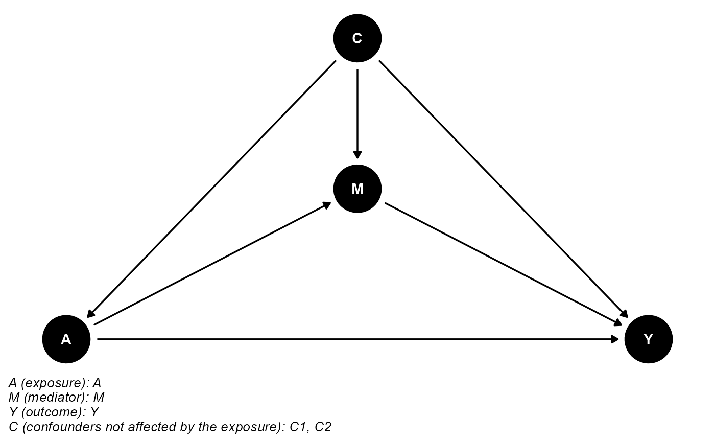
In this setting, we can use all of the six statistical modeling approaches. The results are shown below:
The Regression-based Approach
Closed-form Parameter Function Estimation and Delta Method Inference
res_rb_param_delta <- cmest(data = data, model = "rb", outcome = "Y", exposure = "A",
                            mediator = "M", basec = c("C1", "C2"), EMint = TRUE,
                            mreg = list("logistic"), yreg = "logistic",
                            astar = 0, a = 1, mval = list(1),
                            estimation = "paramfunc", inference = "delta")
summary(res_rb_param_delta)## Causal Mediation Analysis
##
## # Outcome regression:
##
## Call:
## glm(formula = Y ~ A + M + A * M + C1 + C2, family = binomial(),
## data = getCall(x$reg.output$yreg)$data, weights = getCall(x$reg.output$yreg)$weights)
##
## Coefficients:
## Estimate Std. Error z value Pr(>|z|)
## (Intercept) -3.5731 0.7713 -4.633 3.61e-06 ***
## A 0.7084 0.5283 1.341 0.17990
## M -1.0471 0.3736 -2.803 0.00507 **
## C1 0.9337 0.6973 1.339 0.18054
## C2 -0.8415 0.1443 -5.829 5.56e-09 ***
## A:M -0.4222 0.5541 -0.762 0.44607
## ---
## Signif. codes: 0 '***' 0.001 '**' 0.01 '*' 0.05 '.' 0.1 ' ' 1
##
## (Dispersion parameter for binomial family taken to be 1)
##
## Null deviance: 2022.7 on 9999 degrees of freedom
## Residual deviance: 1965.0 on 9994 degrees of freedom
## AIC: 1977
##
## Number of Fisher Scoring iterations: 7
##
##
## # Mediator regressions:
##
## Call:
## glm(formula = M ~ A + C1 + C2, family = binomial(), data = getCall(x$reg.output$mreg[[1L]])$data,
## weights = getCall(x$reg.output$mreg[[1L]])$weights)
##
## Coefficients:
## Estimate Std. Error z value Pr(>|z|)
## (Intercept) 0.4353 0.6410 0.679 0.49712
## A 1.7076 0.1443 11.837 < 2e-16 ***
## C1 1.9982 0.6474 3.086 0.00203 **
## C2 0.9024 0.1345 6.709 1.96e-11 ***
## ---
## Signif. codes: 0 '***' 0.001 '**' 0.01 '*' 0.05 '.' 0.1 ' ' 1
##
## (Dispersion parameter for binomial family taken to be 1)
##
## Null deviance: 2294.0 on 9999 degrees of freedom
## Residual deviance: 2072.5 on 9996 degrees of freedom
## AIC: 2080.5
##
## Number of Fisher Scoring iterations: 7
##
##
## # Effect decomposition on the odds ratio scale via the regression-based approach
##
## Closed-form parameter function estimation with
## delta method standard errors, confidence intervals and p-values
##
## Estimate Std.error 95% CIL 95% CIU P.val
## Rcde 1.33138 0.22278 0.95912 1.848 0.0872 .
## Rpnde 1.41988 0.23708 1.02358 1.970 0.0358 *
## Rtnde 1.34928 0.22056 0.97940 1.859 0.0669 .
## Rpnie 0.93338 0.03576 0.86587 1.006 0.0719 .
## Rtnie 0.88697 0.05295 0.78902 0.997 0.0445 *
## Rte 1.25939 0.19804 0.92535 1.714 0.1425
## ERcde 0.30416 0.20019 -0.08820 0.697 0.1287
## ERintref 0.11571 0.11472 -0.10914 0.341 0.3131
## ERintmed -0.09387 0.09323 -0.27659 0.089 0.3140
## ERpnie -0.06662 0.03576 -0.13670 0.003 0.0624 .
## ERcde(prop) 1.17262 0.23540 0.71124 1.634 6.32e-07 ***
## ERintref(prop) 0.44610 0.49051 -0.51528 1.407 0.3631
## ERintmed(prop) -0.36189 0.39881 -1.14354 0.420 0.3642
## ERpnie(prop) -0.25684 0.23474 -0.71691 0.203 0.2739
## pm -0.61872 0.50289 -1.60437 0.367 0.2186
## int 0.08421 0.09264 -0.09736 0.266 0.3633
## pe -0.17262 0.23540 -0.63400 0.289 0.4634
## ---
## Signif. codes: 0 '***' 0.001 '**' 0.01 '*' 0.05 '.' 0.1 ' ' 1
##
## (Rcde: controlled direct effect odds ratio; Rpnde: pure natural direct effect odds ratio; Rtnde: total natural direct effect odds ratio; Rpnie: pure natural indirect effect odds ratio; Rtnie: total natural indirect effect odds ratio; Rte: total effect odds ratio; ERcde: excess relative risk due to controlled direct effect; ERintref: excess relative risk due to reference interaction; ERintmed: excess relative risk due to mediated interaction; ERpnie: excess relative risk due to pure natural indirect effect; ERcde(prop): proportion ERcde; ERintref(prop): proportion ERintref; ERintmed(prop): proportion ERintmed; ERpnie(prop): proportion ERpnie; pm: overall proportion mediated; int: overall proportion attributable to interaction; pe: overall proportion eliminated)
##
## Relevant variable values:
## $a
## [1] 1
##
## $astar
## [1] 0
##
## $yval
## [1] "1"
##
## $mval
## $mval[[1]]
## [1] 1
##
##
## $basecval
## $basecval[[1]]
## [1] 0.9993463
##
## $basecval[[2]]
## [1] 0.6061Closed-form Parameter Function Estimation and Bootstrap Inference
res_rb_param_bootstrap <- cmest(data = data, model = "rb", outcome = "Y", exposure = "A",
                                mediator = "M", basec = c("C1", "C2"), EMint = TRUE,
                                mreg = list("logistic"), yreg = "logistic",
                                astar = 0, a = 1, mval = list(1),
                                estimation = "paramfunc", inference = "bootstrap", nboot = 2)
summary(res_rb_param_bootstrap)## Causal Mediation Analysis
##
## # Outcome regression:
##
## Call:
## glm(formula = Y ~ A + M + A * M + C1 + C2, family = binomial(),
## data = getCall(x$reg.output$yreg)$data, weights = getCall(x$reg.output$yreg)$weights)
##
## Coefficients:
## Estimate Std. Error z value Pr(>|z|)
## (Intercept) -3.5731 0.7713 -4.633 3.61e-06 ***
## A 0.7084 0.5283 1.341 0.17990
## M -1.0471 0.3736 -2.803 0.00507 **
## C1 0.9337 0.6973 1.339 0.18054
## C2 -0.8415 0.1443 -5.829 5.56e-09 ***
## A:M -0.4222 0.5541 -0.762 0.44607
## ---
## Signif. codes: 0 '***' 0.001 '**' 0.01 '*' 0.05 '.' 0.1 ' ' 1
##
## (Dispersion parameter for binomial family taken to be 1)
##
## Null deviance: 2022.7 on 9999 degrees of freedom
## Residual deviance: 1965.0 on 9994 degrees of freedom
## AIC: 1977
##
## Number of Fisher Scoring iterations: 7
##
##
## # Mediator regressions:
##
## Call:
## glm(formula = M ~ A + C1 + C2, family = binomial(), data = getCall(x$reg.output$mreg[[1L]])$data,
## weights = getCall(x$reg.output$mreg[[1L]])$weights)
##
## Coefficients:
## Estimate Std. Error z value Pr(>|z|)
## (Intercept) 0.4353 0.6410 0.679 0.49712
## A 1.7076 0.1443 11.837 < 2e-16 ***
## C1 1.9982 0.6474 3.086 0.00203 **
## C2 0.9024 0.1345 6.709 1.96e-11 ***
## ---
## Signif. codes: 0 '***' 0.001 '**' 0.01 '*' 0.05 '.' 0.1 ' ' 1
##
## (Dispersion parameter for binomial family taken to be 1)
##
## Null deviance: 2294.0 on 9999 degrees of freedom
## Residual deviance: 2072.5 on 9996 degrees of freedom
## AIC: 2080.5
##
## Number of Fisher Scoring iterations: 7
##
##
## # Effect decomposition on the odds ratio scale via the regression-based approach
##
## Closed-form parameter function estimation with
## bootstrap standard errors, percentile confidence intervals and p-values
##
## Estimate Std.error 95% CIL 95% CIU P.val
## Rcde 1.33138 0.06172 1.14345 1.226 <2e-16 ***
## Rpnde 1.41987 0.19318 1.22863 1.488 <2e-16 ***
## Rtnde 1.34928 0.08947 1.16265 1.283 <2e-16 ***
## Rpnie 0.93338 0.00654 0.90612 0.915 <2e-16 ***
## Rtnie 0.88697 0.05118 0.78870 0.857 <2e-16 ***
## Rte 1.25939 0.08946 1.05350 1.174 <2e-16 ***
## ERcde 0.30416 0.05645 0.12662 0.202 <2e-16 ***
## ERintref 0.11571 0.13672 0.10265 0.286 <2e-16 ***
## ERintmed -0.09387 0.11025 -0.22985 -0.082 <2e-16 ***
## ERpnie -0.06662 0.00654 -0.09388 -0.085 <2e-16 ***
## ERcde(prop) 1.17262 0.92815 1.18783 2.435 <2e-16 ***
## ERintref(prop) 0.44610 0.20645 1.65213 1.929 <2e-16 ***
## ERintmed(prop) -0.36189 0.15593 -1.53545 -1.326 <2e-16 ***
## ERpnie(prop) -0.25684 0.97867 -1.82886 -0.514 <2e-16 ***
## pm -0.61872 1.13460 -3.36430 -1.840 <2e-16 ***
## int 0.08421 0.05052 0.32617 0.394 <2e-16 ***
## pe -0.17262 0.92815 -1.43481 -0.188 <2e-16 ***
## ---
## Signif. codes: 0 '***' 0.001 '**' 0.01 '*' 0.05 '.' 0.1 ' ' 1
##
## (Rcde: controlled direct effect odds ratio; Rpnde: pure natural direct effect odds ratio; Rtnde: total natural direct effect odds ratio; Rpnie: pure natural indirect effect odds ratio; Rtnie: total natural indirect effect odds ratio; Rte: total effect odds ratio; ERcde: excess relative risk due to controlled direct effect; ERintref: excess relative risk due to reference interaction; ERintmed: excess relative risk due to mediated interaction; ERpnie: excess relative risk due to pure natural indirect effect; ERcde(prop): proportion ERcde; ERintref(prop): proportion ERintref; ERintmed(prop): proportion ERintmed; ERpnie(prop): proportion ERpnie; pm: overall proportion mediated; int: overall proportion attributable to interaction; pe: overall proportion eliminated)
##
## Relevant variable values:
## $a
## [1] 1
##
## $astar
## [1] 0
##
## $yval
## [1] "1"
##
## $mval
## $mval[[1]]
## [1] 1
##
##
## $basecval
## $basecval[[1]]
## [1] 0.9993463
##
## $basecval[[2]]
## [1] 0.6061Direct Counterfactual Imputation Estimation and Bootstrap Inference
res_rb_impu_bootstrap <- cmest(data = data, model = "rb", outcome = "Y", exposure = "A",
                               mediator = "M", basec = c("C1", "C2"), EMint = TRUE,
                               mreg = list("logistic"), yreg = "logistic",
                               astar = 0, a = 1, mval = list(1),
                               estimation = "imputation", inference = "bootstrap", nboot = 2)
summary(res_rb_impu_bootstrap)## Causal Mediation Analysis
##
## # Outcome regression:
##
## Call:
## glm(formula = Y ~ A + M + A * M + C1 + C2, family = binomial(),
## data = getCall(x$reg.output$yreg)$data, weights = getCall(x$reg.output$yreg)$weights)
##
## Coefficients:
## Estimate Std. Error z value Pr(>|z|)
## (Intercept) -3.5731 0.7713 -4.633 3.61e-06 ***
## A 0.7084 0.5283 1.341 0.17990
## M -1.0471 0.3736 -2.803 0.00507 **
## C1 0.9337 0.6973 1.339 0.18054
## C2 -0.8415 0.1443 -5.829 5.56e-09 ***
## A:M -0.4222 0.5541 -0.762 0.44607
## ---
## Signif. codes: 0 '***' 0.001 '**' 0.01 '*' 0.05 '.' 0.1 ' ' 1
##
## (Dispersion parameter for binomial family taken to be 1)
##
## Null deviance: 2022.7 on 9999 degrees of freedom
## Residual deviance: 1965.0 on 9994 degrees of freedom
## AIC: 1977
##
## Number of Fisher Scoring iterations: 7
##
##
## # Mediator regressions:
##
## Call:
## glm(formula = M ~ A + C1 + C2, family = binomial(), data = getCall(x$reg.output$mreg[[1L]])$data,
## weights = getCall(x$reg.output$mreg[[1L]])$weights)
##
## Coefficients:
## Estimate Std. Error z value Pr(>|z|)
## (Intercept) 0.4353 0.6410 0.679 0.49712
## A 1.7076 0.1443 11.837 < 2e-16 ***
## C1 1.9982 0.6474 3.086 0.00203 **
## C2 0.9024 0.1345 6.709 1.96e-11 ***
## ---
## Signif. codes: 0 '***' 0.001 '**' 0.01 '*' 0.05 '.' 0.1 ' ' 1
##
## (Dispersion parameter for binomial family taken to be 1)
##
## Null deviance: 2294.0 on 9999 degrees of freedom
## Residual deviance: 2072.5 on 9996 degrees of freedom
## AIC: 2080.5
##
## Number of Fisher Scoring iterations: 7
##
##
## # Effect decomposition on the odds ratio scale via the regression-based approach
##
## Direct counterfactual imputation estimation with
## bootstrap standard errors, percentile confidence intervals and p-values
##
## Estimate Std.error 95% CIL 95% CIU P.val
## Rcde 1.330044 0.009511 1.257553 1.270 <2e-16 ***
## Rpnde 1.420177 0.137613 1.364635 1.550 <2e-16 ***
## Rtnde 1.349577 0.011604 1.288417 1.304 <2e-16 ***
## Rpnie 0.924473 0.003410 0.912807 0.917 <2e-16 ***
## Rtnie 0.878515 0.072922 0.768186 0.866 <2e-16 ***
## Rte 1.247647 0.006199 1.181979 1.190 <2e-16 ***
## ERcde 0.292988 0.008426 0.226739 0.238 <2e-16 ***
## ERintref 0.127190 0.146039 0.126886 0.323 <2e-16 ***
## ERintmed -0.097003 0.128004 -0.272328 -0.100 <2e-16 ***
## ERpnie -0.075527 0.003410 -0.087192 -0.083 <2e-16 ***
## ERcde(prop) 1.183086 0.086892 1.191564 1.308 <2e-16 ***
## ERintref(prop) 0.513593 0.744711 0.696016 1.697 <2e-16 ***
## ERintmed(prop) -0.391700 0.654687 -1.429943 -0.550 <2e-16 ***
## ERpnie(prop) -0.304980 0.003131 -0.458158 -0.454 <2e-16 ***
## pm -0.696679 0.657819 -1.888101 -1.004 <2e-16 ***
## int 0.121894 0.090024 0.145647 0.267 <2e-16 ***
## pe -0.183086 0.086892 -0.308304 -0.192 <2e-16 ***
## ---
## Signif. codes: 0 '***' 0.001 '**' 0.01 '*' 0.05 '.' 0.1 ' ' 1
##
## (Rcde: controlled direct effect odds ratio; Rpnde: pure natural direct effect odds ratio; Rtnde: total natural direct effect odds ratio; Rpnie: pure natural indirect effect odds ratio; Rtnie: total natural indirect effect odds ratio; Rte: total effect odds ratio; ERcde: excess relative risk due to controlled direct effect; ERintref: excess relative risk due to reference interaction; ERintmed: excess relative risk due to mediated interaction; ERpnie: excess relative risk due to pure natural indirect effect; ERcde(prop): proportion ERcde; ERintref(prop): proportion ERintref; ERintmed(prop): proportion ERintmed; ERpnie(prop): proportion ERpnie; pm: overall proportion mediated; int: overall proportion attributable to interaction; pe: overall proportion eliminated)
##
## Relevant variable values:
## $a
## [1] 1
##
## $astar
## [1] 0
##
## $yval
## [1] "1"
##
## $mval
## $mval[[1]]
## [1] 1The Weighting-based Approach
res_wb <- cmest(data = data, model = "wb", outcome = "Y", exposure = "A",
                mediator = "M", basec = c("C1", "C2"), EMint = TRUE,
                ereg = "logistic", yreg = "logistic",
                astar = 0, a = 1, mval = list(1),
                estimation = "imputation", inference = "bootstrap", nboot = 2)
summary(res_wb)## Causal Mediation Analysis
##
## # Outcome regression:
##
## Call:
## glm(formula = Y ~ A + M + A * M + C1 + C2, family = binomial(),
## data = getCall(x$reg.output$yreg)$data, weights = getCall(x$reg.output$yreg)$weights)
##
## Coefficients:
## Estimate Std. Error z value Pr(>|z|)
## (Intercept) -3.5731 0.7713 -4.633 3.61e-06 ***
## A 0.7084 0.5283 1.341 0.17990
## M -1.0471 0.3736 -2.803 0.00507 **
## C1 0.9337 0.6973 1.339 0.18054
## C2 -0.8415 0.1443 -5.829 5.56e-09 ***
## A:M -0.4222 0.5541 -0.762 0.44607
## ---
## Signif. codes: 0 '***' 0.001 '**' 0.01 '*' 0.05 '.' 0.1 ' ' 1
##
## (Dispersion parameter for binomial family taken to be 1)
##
## Null deviance: 2022.7 on 9999 degrees of freedom
## Residual deviance: 1965.0 on 9994 degrees of freedom
## AIC: 1977
##
## Number of Fisher Scoring iterations: 7
##
##
## # Exposure regression for weighting:
##
## Call:
## glm(formula = A ~ C1 + C2, family = binomial(), data = getCall(x$reg.output$ereg)$data,
## weights = getCall(x$reg.output$ereg)$weights)
##
## Coefficients:
## Estimate Std. Error z value Pr(>|z|)
## (Intercept) 0.08342 0.21440 0.389 0.69723
## C1 0.60899 0.21208 2.872 0.00409 **
## C2 0.10532 0.04375 2.407 0.01606 *
## ---
## Signif. codes: 0 '***' 0.001 '**' 0.01 '*' 0.05 '.' 0.1 ' ' 1
##
## (Dispersion parameter for binomial family taken to be 1)
##
## Null deviance: 12534 on 9999 degrees of freedom
## Residual deviance: 12520 on 9997 degrees of freedom
## AIC: 12526
##
## Number of Fisher Scoring iterations: 4
##
##
## # Effect decomposition on the odds ratio scale via the weighting-based approach
##
## Direct counterfactual imputation estimation with
## bootstrap standard errors, percentile confidence intervals and p-values
##
## Estimate Std.error 95% CIL 95% CIU P.val
## Rcde 1.33004 0.19217 0.96491 1.223 1
## Rpnde 1.42603 0.12670 1.16844 1.339 <2e-16 ***
## Rtnde 1.35033 0.18078 1.00664 1.249 <2e-16 ***
## Rpnie 0.92151 0.03436 0.93377 0.980 <2e-16 ***
## Rtnie 0.87259 0.02034 0.84425 0.872 <2e-16 ***
## Rte 1.24434 0.13420 0.98645 1.167 1
## ERcde 0.29184 0.17394 -0.03315 0.201 1
## ERintref 0.13419 0.04724 0.13843 0.202 <2e-16 ***
## ERintmed -0.10320 0.04186 -0.16187 -0.106 <2e-16 ***
## ERpnie -0.07849 0.03436 -0.06620 -0.020 <2e-16 ***
## ERcde(prop) 1.19441 0.70245 1.22728 2.171 <2e-16 ***
## ERintref(prop) 0.54919 8.60458 -11.06885 0.491 1
## ERintmed(prop) -0.42236 6.88147 -0.36260 8.883 1
## ERpnie(prop) -0.32123 1.02066 -0.35611 1.015 1
## pm -0.74359 7.90213 -0.71871 9.898 1
## int 0.12682 1.72311 -2.18618 0.129 1
## pe -0.19441 0.70245 -1.17102 -0.227 <2e-16 ***
## ---
## Signif. codes: 0 '***' 0.001 '**' 0.01 '*' 0.05 '.' 0.1 ' ' 1
##
## (Rcde: controlled direct effect odds ratio; Rpnde: pure natural direct effect odds ratio; Rtnde: total natural direct effect odds ratio; Rpnie: pure natural indirect effect odds ratio; Rtnie: total natural indirect effect odds ratio; Rte: total effect odds ratio; ERcde: excess relative risk due to controlled direct effect; ERintref: excess relative risk due to reference interaction; ERintmed: excess relative risk due to mediated interaction; ERpnie: excess relative risk due to pure natural indirect effect; ERcde(prop): proportion ERcde; ERintref(prop): proportion ERintref; ERintmed(prop): proportion ERintmed; ERpnie(prop): proportion ERpnie; pm: overall proportion mediated; int: overall proportion attributable to interaction; pe: overall proportion eliminated)
##
## Relevant variable values:
## $a
## [1] 1
##
## $astar
## [1] 0
##
## $yval
## [1] "1"
##
## $mval
## $mval[[1]]
## [1] 1The Inverse Odds-ratio Weighting Approach
res_iorw <- cmest(data = data, model = "iorw", outcome = "Y", exposure = "A",
                  mediator = "M", basec = c("C1", "C2"),
                  ereg = "logistic", yreg = "logistic",
                  astar = 0, a = 1, mval = list(1),
                  estimation = "imputation", inference = "bootstrap", nboot = 2)
summary(res_iorw)## Causal Mediation Analysis
##
## # Outcome regression for the total effect:
##
## Call:
## glm(formula = Y ~ A + C1 + C2, family = binomial(), data = getCall(x$reg.output$yregTot)$data,
## weights = getCall(x$reg.output$yregTot)$weights)
##
## Coefficients:
## Estimate Std. Error z value Pr(>|z|)
## (Intercept) -4.4182 0.7137 -6.191 5.98e-10 ***
## A 0.2183 0.1565 1.395 0.163
## C1 0.8540 0.6956 1.228 0.220
## C2 -0.8831 0.1435 -6.156 7.47e-10 ***
## ---
## Signif. codes: 0 '***' 0.001 '**' 0.01 '*' 0.05 '.' 0.1 ' ' 1
##
## (Dispersion parameter for binomial family taken to be 1)
##
## Null deviance: 2022.7 on 9999 degrees of freedom
## Residual deviance: 1980.4 on 9996 degrees of freedom
## AIC: 1988.4
##
## Number of Fisher Scoring iterations: 7
##
##
## # Outcome regression for the direct effect:
##
## Call:
## glm(formula = Y ~ A + C1 + C2, family = binomial(), data = getCall(x$reg.output$yregDir)$data,
## weights = getCall(x$reg.output$yregDir)$weights)
##
## Coefficients:
## Estimate Std. Error z value Pr(>|z|)
## (Intercept) -3.7823 0.8563 -4.417 1.00e-05 ***
## A 0.3675 0.1735 2.118 0.0342 *
## C1 0.2839 0.8440 0.336 0.7366
## C2 -1.0638 0.1803 -5.901 3.61e-09 ***
## ---
## Signif. codes: 0 '***' 0.001 '**' 0.01 '*' 0.05 '.' 0.1 ' ' 1
##
## (Dispersion parameter for binomial family taken to be 1)
##
## Null deviance: 1354.8 on 9999 degrees of freedom
## Residual deviance: 1312.7 on 9996 degrees of freedom
## AIC: 798.25
##
## Number of Fisher Scoring iterations: 7
##
##
## # Exposure regression for weighting:
##
## Call:
## glm(formula = A ~ M + C1 + C2, family = binomial(), data = getCall(x$reg.output$ereg)$data,
## weights = getCall(x$reg.output$ereg)$weights)
##
## Coefficients:
## Estimate Std. Error z value Pr(>|z|)
## (Intercept) -1.4666 0.2542 -5.770 7.91e-09 ***
## M 1.7067 0.1442 11.832 < 2e-16 ***
## C1 0.5218 0.2140 2.438 0.0148 *
## C2 0.0648 0.0443 1.463 0.1436
## ---
## Signif. codes: 0 '***' 0.001 '**' 0.01 '*' 0.05 '.' 0.1 ' ' 1
##
## (Dispersion parameter for binomial family taken to be 1)
##
## Null deviance: 12534 on 9999 degrees of freedom
## Residual deviance: 12360 on 9996 degrees of freedom
## AIC: 12368
##
## Number of Fisher Scoring iterations: 4
##
##
## # Effect decomposition on the odds ratio scale via the inverse odds ratio weighting approach
##
## Direct counterfactual imputation estimation with
## bootstrap standard errors, percentile confidence intervals and p-values
##
## Estimate Std.error 95% CIL 95% CIU P.val
## Rte 1.24287 0.12206 1.34981 1.514 <2e-16 ***
## Rpnde 1.44092 0.26158 1.43458 1.786 <2e-16 ***
## Rtnie 0.86256 0.06944 0.84762 0.941 <2e-16 ***
## pm -0.81541 0.21427 -0.52853 -0.241 <2e-16 ***
## ---
## Signif. codes: 0 '***' 0.001 '**' 0.01 '*' 0.05 '.' 0.1 ' ' 1
##
## (Rte: total effect odds ratio; Rpnde: pure natural direct effect odds ratio; Rtnie: total natural indirect effect odds ratio; pm: proportion mediated)
##
## Relevant variable values:
## $a
## [1] 1
##
## $astar
## [1] 0
##
## $yval
## [1] "1"
{r message=F,warning=F,results='hide'} # res_ne <- cmest(data = data, model = "ne", outcome = "Y", exposure = "A", # mediator = "M", basec = c("C1", "C2"), EMint = TRUE, # yreg = "logistic", # astar = 0, a = 1, mval = list(1), # estimation = "imputation", inference = "bootstrap", nboot = 2) #
{r message=F,warning=F} # summary(res_ne) #
The Marginal Structural Model
res_msm <- cmest(data = data, model = "msm", outcome = "Y", exposure = "A",
                 mediator = "M", basec = c("C1", "C2"), EMint = TRUE,
                 ereg = "logistic", yreg = "logistic", mreg = list("logistic"),
                 wmnomreg = list("logistic"), wmdenomreg = list("logistic"),
                 astar = 0, a = 1, mval = list(1),
                 estimation = "imputation", inference = "bootstrap", nboot = 2)
summary(res_msm)## Causal Mediation Analysis
##
## # Outcome regression:
##
## Call:
## glm(formula = Y ~ A + M + A * M, family = binomial(), data = getCall(x$reg.output$yreg)$data,
## weights = getCall(x$reg.output$yreg)$weights)
##
## Coefficients:
## Estimate Std. Error z value Pr(>|z|)
## (Intercept) -3.1163 0.3762 -8.284 <2e-16 ***
## A 0.4632 0.6200 0.747 0.4550
## M -0.9908 0.4028 -2.460 0.0139 *
## A:M -0.1803 0.6421 -0.281 0.7789
## ---
## Signif. codes: 0 '***' 0.001 '**' 0.01 '*' 0.05 '.' 0.1 ' ' 1
##
## (Dispersion parameter for binomial family taken to be 1)
##
## Null deviance: 1996.3 on 9999 degrees of freedom
## Residual deviance: 1985.5 on 9996 degrees of freedom
## AIC: 2014.4
##
## Number of Fisher Scoring iterations: 6
##
##
## # Mediator regressions:
##
## Call:
## glm(formula = M ~ A, family = binomial(), data = getCall(x$reg.output$mreg[[1L]])$data,
## weights = getCall(x$reg.output$mreg[[1L]])$weights)
##
## Coefficients:
## Estimate Std. Error z value Pr(>|z|)
## (Intercept) 2.87310 0.07858 36.56 <2e-16 ***
## A 1.69598 0.14370 11.80 <2e-16 ***
## ---
## Signif. codes: 0 '***' 0.001 '**' 0.01 '*' 0.05 '.' 0.1 ' ' 1
##
## (Dispersion parameter for binomial family taken to be 1)
##
## Null deviance: 2271.0 on 9999 degrees of freedom
## Residual deviance: 2112.9 on 9998 degrees of freedom
## AIC: 2132.1
##
## Number of Fisher Scoring iterations: 7
##
##
## # Mediator regressions for weighting (denominator):
##
## Call:
## glm(formula = M ~ A + C1 + C2, family = binomial(), data = getCall(x$reg.output$wmdenomreg[[1L]])$data,
## weights = getCall(x$reg.output$wmdenomreg[[1L]])$weights)
##
## Coefficients:
## Estimate Std. Error z value Pr(>|z|)
## (Intercept) 0.4353 0.6410 0.679 0.49712
## A 1.7076 0.1443 11.837 < 2e-16 ***
## C1 1.9982 0.6474 3.086 0.00203 **
## C2 0.9024 0.1345 6.709 1.96e-11 ***
## ---
## Signif. codes: 0 '***' 0.001 '**' 0.01 '*' 0.05 '.' 0.1 ' ' 1
##
## (Dispersion parameter for binomial family taken to be 1)
##
## Null deviance: 2294.0 on 9999 degrees of freedom
## Residual deviance: 2072.5 on 9996 degrees of freedom
## AIC: 2080.5
##
## Number of Fisher Scoring iterations: 7
##
##
## # Mediator regressions for weighting (nominator):
##
## Call:
## glm(formula = M ~ A, family = binomial(), data = getCall(x$reg.output$wmnomreg[[1L]])$data,
## weights = getCall(x$reg.output$wmnomreg[[1L]])$weights)
##
## Coefficients:
## Estimate Std. Error z value Pr(>|z|)
## (Intercept) 2.84922 0.07775 36.65 <2e-16 ***
## A 1.73145 0.14383 12.04 <2e-16 ***
## ---
## Signif. codes: 0 '***' 0.001 '**' 0.01 '*' 0.05 '.' 0.1 ' ' 1
##
## (Dispersion parameter for binomial family taken to be 1)
##
## Null deviance: 2294 on 9999 degrees of freedom
## Residual deviance: 2128 on 9998 degrees of freedom
## AIC: 2132
##
## Number of Fisher Scoring iterations: 7
##
##
## # Exposure regression for weighting:
##
## Call:
## glm(formula = A ~ C1 + C2, family = binomial(), data = getCall(x$reg.output$ereg)$data,
## weights = getCall(x$reg.output$ereg)$weights)
##
## Coefficients:
## Estimate Std. Error z value Pr(>|z|)
## (Intercept) 0.08342 0.21440 0.389 0.69723
## C1 0.60899 0.21208 2.872 0.00409 **
## C2 0.10532 0.04375 2.407 0.01606 *
## ---
## Signif. codes: 0 '***' 0.001 '**' 0.01 '*' 0.05 '.' 0.1 ' ' 1
##
## (Dispersion parameter for binomial family taken to be 1)
##
## Null deviance: 12534 on 9999 degrees of freedom
## Residual deviance: 12520 on 9997 degrees of freedom
## AIC: 12526
##
## Number of Fisher Scoring iterations: 4
##
##
## # Effect decomposition on the odds ratio scale via the marginal structural model
##
## Direct counterfactual imputation estimation with
## bootstrap standard errors, percentile confidence intervals and p-values
##
## Estimate Std.error 95% CIL 95% CIU P.val
## Rcde 1.326939 0.024278 1.520315 1.553 <2e-16 ***
## Rpnde 1.357747 0.018355 1.525370 1.550 <2e-16 ***
## Rtnde 1.333507 0.014825 1.526419 1.546 <2e-16 ***
## Rpnie 0.936022 0.018089 0.887888 0.912 <2e-16 ***
## Rtnie 0.919311 0.001338 0.898296 0.900 <2e-16 ***
## Rte 1.248192 0.014448 1.372974 1.392 <2e-16 ***
## ERcde 0.294772 0.006927 0.455193 0.464 <2e-16 ***
## ERintref 0.062975 0.025282 0.060876 0.095 <2e-16 ***
## ERintmed -0.045577 0.021996 -0.069846 -0.040 <2e-16 ***
## ERpnie -0.063978 0.018089 -0.112103 -0.088 <2e-16 ***
## ERcde(prop) 1.187675 0.063512 1.160170 1.245 <2e-16 ***
## ERintref(prop) 0.253737 0.058425 0.163106 0.242 <2e-16 ***
## ERintmed(prop) -0.183636 0.052083 -0.177908 -0.108 <2e-16 ***
## ERpnie(prop) -0.257775 0.057170 -0.300670 -0.224 <2e-16 ***
## pm -0.441412 0.005087 -0.408605 -0.402 <2e-16 ***
## int 0.070100 0.006342 0.055172 0.064 <2e-16 ***
## pe -0.187675 0.063512 -0.245499 -0.160 <2e-16 ***
## ---
## Signif. codes: 0 '***' 0.001 '**' 0.01 '*' 0.05 '.' 0.1 ' ' 1
##
## (Rcde: controlled direct effect odds ratio; Rpnde: pure natural direct effect odds ratio; Rtnde: total natural direct effect odds ratio; Rpnie: pure natural indirect effect odds ratio; Rtnie: total natural indirect effect odds ratio; Rte: total effect odds ratio; ERcde: excess relative risk due to controlled direct effect; ERintref: excess relative risk due to reference interaction; ERintmed: excess relative risk due to mediated interaction; ERpnie: excess relative risk due to pure natural indirect effect; ERcde(prop): proportion ERcde; ERintref(prop): proportion ERintref; ERintmed(prop): proportion ERintmed; ERpnie(prop): proportion ERpnie; pm: overall proportion mediated; int: overall proportion attributable to interaction; pe: overall proportion eliminated)
##
## Relevant variable values:
## $a
## [1] 1
##
## $astar
## [1] 0
##
## $yval
## [1] "1"
##
## $mval
## $mval[[1]]
## [1] 1The g-formula Approach
res_gformula <- cmest(data = data, model = "gformula", outcome = "Y", exposure = "A",
                      mediator = "M", basec = c("C1", "C2"), EMint = TRUE,
                      mreg = list("logistic"), yreg = "logistic",
                      astar = 0, a = 1, mval = list(1),
                      estimation = "imputation", inference = "bootstrap", nboot = 2)
summary(res_gformula)## Causal Mediation Analysis
##
## # Outcome regression:
##
## Call:
## glm(formula = Y ~ A + M + A * M + C1 + C2, family = binomial(),
## data = getCall(x$reg.output$yreg)$data, weights = getCall(x$reg.output$yreg)$weights)
##
## Coefficients:
## Estimate Std. Error z value Pr(>|z|)
## (Intercept) -3.5731 0.7713 -4.633 3.61e-06 ***
## A 0.7084 0.5283 1.341 0.17990
## M -1.0471 0.3736 -2.803 0.00507 **
## C1 0.9337 0.6973 1.339 0.18054
## C2 -0.8415 0.1443 -5.829 5.56e-09 ***
## A:M -0.4222 0.5541 -0.762 0.44607
## ---
## Signif. codes: 0 '***' 0.001 '**' 0.01 '*' 0.05 '.' 0.1 ' ' 1
##
## (Dispersion parameter for binomial family taken to be 1)
##
## Null deviance: 2022.7 on 9999 degrees of freedom
## Residual deviance: 1965.0 on 9994 degrees of freedom
## AIC: 1977
##
## Number of Fisher Scoring iterations: 7
##
##
## # Mediator regressions:
##
## Call:
## glm(formula = M ~ A + C1 + C2, family = binomial(), data = getCall(x$reg.output$mreg[[1L]])$data,
## weights = getCall(x$reg.output$mreg[[1L]])$weights)
##
## Coefficients:
## Estimate Std. Error z value Pr(>|z|)
## (Intercept) 0.4353 0.6410 0.679 0.49712
## A 1.7076 0.1443 11.837 < 2e-16 ***
## C1 1.9982 0.6474 3.086 0.00203 **
## C2 0.9024 0.1345 6.709 1.96e-11 ***
## ---
## Signif. codes: 0 '***' 0.001 '**' 0.01 '*' 0.05 '.' 0.1 ' ' 1
##
## (Dispersion parameter for binomial family taken to be 1)
##
## Null deviance: 2294.0 on 9999 degrees of freedom
## Residual deviance: 2072.5 on 9996 degrees of freedom
## AIC: 2080.5
##
## Number of Fisher Scoring iterations: 7
##
##
## # Effect decomposition on the odds ratio scale via the g-formula approach
##
## Direct counterfactual imputation estimation with
## bootstrap standard errors, percentile confidence intervals and p-values
##
## Estimate Std.error 95% CIL 95% CIU P.val
## Rcde 1.330044 0.277865 0.988256 1.361 1
## Rpnde 1.421621 0.194347 1.124066 1.385 <2e-16 ***
## Rtnde 1.351145 0.255814 1.022707 1.366 <2e-16 ***
## Rpnie 0.924490 0.044053 0.886909 0.946 <2e-16 ***
## Rtnie 0.878659 0.010460 0.860782 0.875 <2e-16 ***
## Rte 1.249120 0.181787 0.967576 1.212 1
## ERcde 0.292480 0.236163 -0.009933 0.307 1
## ERintref 0.129141 0.041816 0.078530 0.135 <2e-16 ***
## ERintmed -0.096991 0.031493 -0.102632 -0.060 <2e-16 ***
## ERpnie -0.075510 0.044053 -0.113040 -0.054 <2e-16 ***
## ERcde(prop) 1.174052 0.680590 0.503465 1.418 <2e-16 ***
## ERintref(prop) 0.518391 2.773970 -3.472994 0.254 1
## ERintmed(prop) -0.389334 2.114797 -0.195649 2.646 1
## ERpnie(prop) -0.303108 1.339763 -0.476034 1.324 1
## pm -0.692443 3.454560 -0.671683 3.970 1
## int 0.129057 0.659174 -0.827408 0.058 1
## pe -0.174052 0.680590 -0.417840 0.497 1
## ---
## Signif. codes: 0 '***' 0.001 '**' 0.01 '*' 0.05 '.' 0.1 ' ' 1
##
## (Rcde: controlled direct effect odds ratio; Rpnde: pure natural direct effect odds ratio; Rtnde: total natural direct effect odds ratio; Rpnie: pure natural indirect effect odds ratio; Rtnie: total natural indirect effect odds ratio; Rte: total effect odds ratio; ERcde: excess relative risk due to controlled direct effect; ERintref: excess relative risk due to reference interaction; ERintmed: excess relative risk due to mediated interaction; ERpnie: excess relative risk due to pure natural indirect effect; ERcde(prop): proportion ERcde; ERintref(prop): proportion ERintref; ERintmed(prop): proportion ERintmed; ERpnie(prop): proportion ERpnie; pm: overall proportion mediated; int: overall proportion attributable to interaction; pe: overall proportion eliminated)
##
## Relevant variable values:
## $a
## [1] 1
##
## $astar
## [1] 0
##
## $yval
## [1] "1"
##
## $mval
## $mval[[1]]
## [1] 1