Multiple Imputations with Missing Data
2025-12-08
Source:vignettes/multiple_imputation.Rmd
multiple_imputation.RmdThis example demonstrates how to estimate causal effects with
multiple imputations by using cmest when the dataset
contains missing values. For this purpose, we simulate some data
containing a continuous baseline confounder
,
a binary baseline confounder
,
a binary exposure
,
a binary mediator
and a binary outcome
.
The true regression models for
,
and
are:
To create the dataset with missing values, we randomly delete 10% of values in the dataset.
set.seed(1)
expit <- function(x) exp(x)/(1+exp(x))
n <- 10000
C1 <- rnorm(n, mean = 1, sd = 0.1)
C2 <- rbinom(n, 1, 0.6)
A <- rbinom(n, 1, expit(0.2 + 0.5*C1 + 0.1*C2))
M <- rbinom(n, 1, expit(1 + 2*A + 1.5*C1 + 0.8*C2))
Y <- rbinom(n, 1, expit(-3 - 0.4*A - 1.2*M + 0.5*A*M + 0.3*C1 - 0.6*C2))
data_noNA <- data.frame(A, M, Y, C1, C2)
missing <- sample(1:(5*n), n*0.1, replace = FALSE)
C1[missing[which(missing <= n)]] <- NA
C2[missing[which((missing > n)*(missing <= 2*n) == 1)] - n] <- NA
A[missing[which((missing > 2*n)*(missing <= 3*n) == 1)] - 2*n] <- NA
M[missing[which((missing > 3*n)*(missing <= 4*n) == 1)] - 3*n] <- NA
Y[missing[which((missing > 4*n)*(missing <= 5*n) == 1)] - 4*n] <- NA
data <- data.frame(A, M, Y, C1, C2)
The DAG for this scientific setting is:
library(CMAverse)
cmdag(outcome = "Y", exposure = "A", mediator = "M",
      basec = c("C1", "C2"), postc = NULL, node = TRUE, text_col = "white")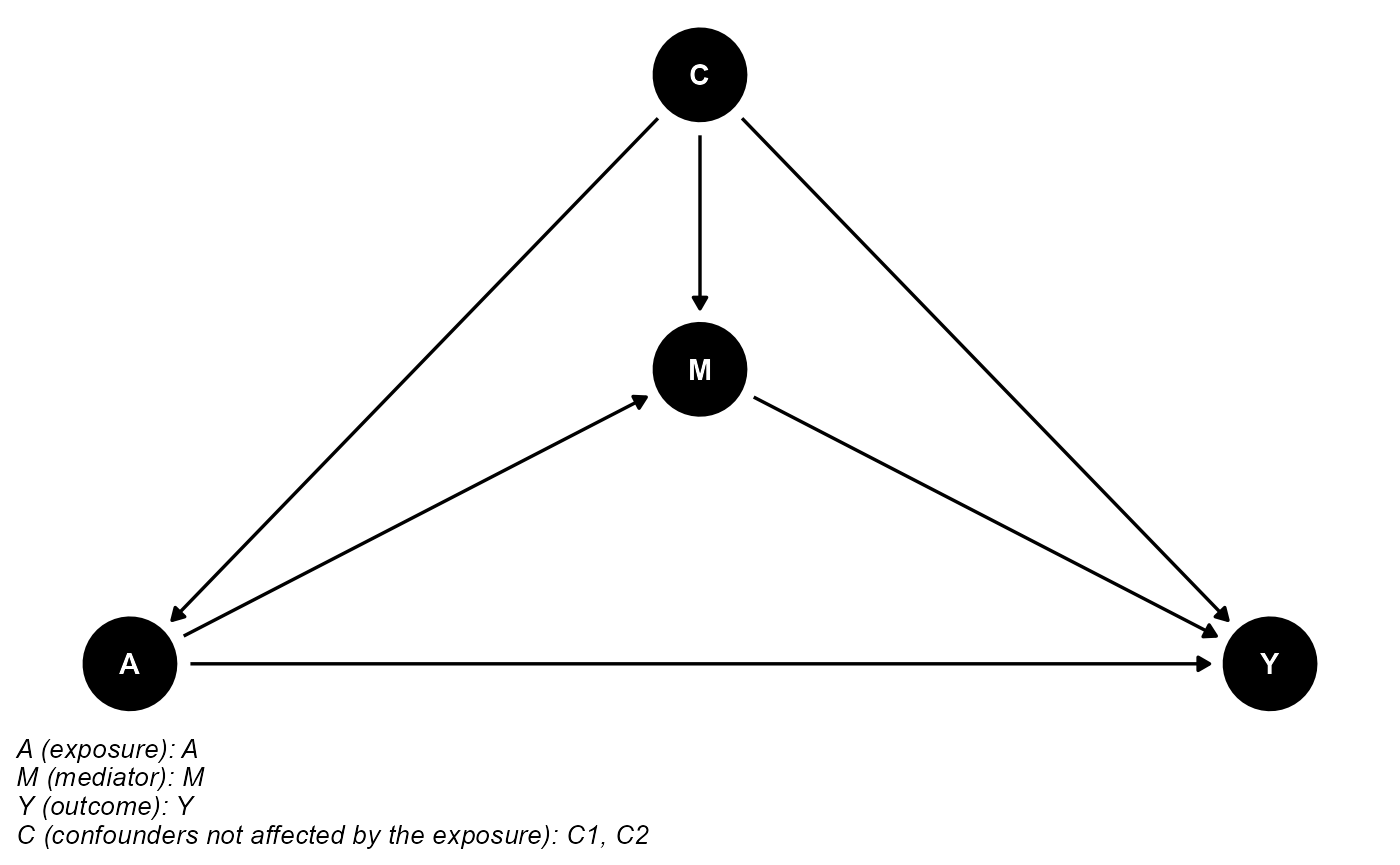
To conduct multiple imputations, we set the multimp
argument to be TRUE. The regression-based approach is used
for illustration. The multiple imputation results:
res_multimp <- cmest(data = data, model = "rb", outcome = "Y", exposure = "A",
                     mediator = "M", basec = c("C1", "C2"), EMint = TRUE,
                     mreg = list("logistic"), yreg = "logistic",
                     astar = 0, a = 1, mval = list(1),
                     estimation = "paramfunc", inference = "delta",
                     multimp = TRUE, args_mice = list(m = 10))
summary(res_multimp)## Causal Mediation Analysis
##
## # Regressions with imputed dataset 1
##
## ## Outcome regression:
##
## Call:
## glm(formula = Y ~ A + M + A * M + C1 + C2, family = binomial(),
## data = getCall(x$reg.output[[1L]]$yreg)$data, weights = getCall(x$reg.output[[1L]]$yreg)$weights)
##
## Coefficients:
## Estimate Std. Error z value Pr(>|z|)
## (Intercept) -3.2073 0.7749 -4.139 3.49e-05 ***
## A 0.6995 0.5285 1.324 0.18566
## M -1.1032 0.3747 -2.944 0.00324 **
## C1 0.5753 0.7042 0.817 0.41398
## C2 -0.8395 0.1452 -5.782 7.38e-09 ***
## A:M -0.3609 0.5552 -0.650 0.51560
## ---
## Signif. codes: 0 '***' 0.001 '**' 0.01 '*' 0.05 '.' 0.1 ' ' 1
##
## (Dispersion parameter for binomial family taken to be 1)
##
## Null deviance: 2007.3 on 9999 degrees of freedom
## Residual deviance: 1949.7 on 9994 degrees of freedom
## AIC: 1961.7
##
## Number of Fisher Scoring iterations: 7
##
##
## ## Mediator regressions:
##
## Call:
## glm(formula = M ~ A + C1 + C2, family = binomial(), data = getCall(x$reg.output[[1L]]$mreg[[1L]])$data,
## weights = getCall(x$reg.output[[1L]]$mreg[[1L]])$weights)
##
## Coefficients:
## Estimate Std. Error z value Pr(>|z|)
## (Intercept) 0.2581 0.6480 0.398 0.690438
## A 1.7239 0.1459 11.817 < 2e-16 ***
## C1 2.1778 0.6550 3.325 0.000884 ***
## C2 0.9341 0.1358 6.876 6.15e-12 ***
## ---
## Signif. codes: 0 '***' 0.001 '**' 0.01 '*' 0.05 '.' 0.1 ' ' 1
##
## (Dispersion parameter for binomial family taken to be 1)
##
## Null deviance: 2271.9 on 9999 degrees of freedom
## Residual deviance: 2045.9 on 9996 degrees of freedom
## AIC: 2053.9
##
## Number of Fisher Scoring iterations: 7
##
##
## # Regressions with imputed dataset 2
##
## ## Outcome regression:
##
## Call:
## glm(formula = Y ~ A + M + A * M + C1 + C2, family = binomial(),
## data = getCall(x$reg.output[[2L]]$yreg)$data, weights = getCall(x$reg.output[[2L]]$yreg)$weights)
##
## Coefficients:
## Estimate Std. Error z value Pr(>|z|)
## (Intercept) -3.2236 0.7618 -4.232 2.32e-05 ***
## A 0.5370 0.5176 1.037 0.29955
## M -1.1753 0.3586 -3.277 0.00105 **
## C1 0.7233 0.6970 1.038 0.29935
## C2 -0.8819 0.1449 -6.085 1.17e-09 ***
## A:M -0.2414 0.5441 -0.444 0.65724
## ---
## Signif. codes: 0 '***' 0.001 '**' 0.01 '*' 0.05 '.' 0.1 ' ' 1
##
## (Dispersion parameter for binomial family taken to be 1)
##
## Null deviance: 2030.4 on 9999 degrees of freedom
## Residual deviance: 1967.8 on 9994 degrees of freedom
## AIC: 1979.8
##
## Number of Fisher Scoring iterations: 7
##
##
## ## Mediator regressions:
##
## Call:
## glm(formula = M ~ A + C1 + C2, family = binomial(), data = getCall(x$reg.output[[2L]]$mreg[[1L]])$data,
## weights = getCall(x$reg.output[[2L]]$mreg[[1L]])$weights)
##
## Coefficients:
## Estimate Std. Error z value Pr(>|z|)
## (Intercept) 0.2210 0.6469 0.342 0.732665
## A 1.6816 0.1447 11.625 < 2e-16 ***
## C1 2.2165 0.6546 3.386 0.000709 ***
## C2 0.9660 0.1364 7.082 1.42e-12 ***
## ---
## Signif. codes: 0 '***' 0.001 '**' 0.01 '*' 0.05 '.' 0.1 ' ' 1
##
## (Dispersion parameter for binomial family taken to be 1)
##
## Null deviance: 2271.9 on 9999 degrees of freedom
## Residual deviance: 2048.3 on 9996 degrees of freedom
## AIC: 2056.3
##
## Number of Fisher Scoring iterations: 7
##
##
## # Regressions with imputed dataset 3
##
## ## Outcome regression:
##
## Call:
## glm(formula = Y ~ A + M + A * M + C1 + C2, family = binomial(),
## data = getCall(x$reg.output[[3L]]$yreg)$data, weights = getCall(x$reg.output[[3L]]$yreg)$weights)
##
## Coefficients:
## Estimate Std. Error z value Pr(>|z|)
## (Intercept) -3.4344 0.7709 -4.455 8.38e-06 ***
## A 0.7089 0.5289 1.340 0.18015
## M -1.0578 0.3738 -2.830 0.00465 **
## C1 0.8036 0.6991 1.150 0.25035
## C2 -0.8491 0.1451 -5.853 4.83e-09 ***
## A:M -0.4207 0.5548 -0.758 0.44829
## ---
## Signif. codes: 0 '***' 0.001 '**' 0.01 '*' 0.05 '.' 0.1 ' ' 1
##
## (Dispersion parameter for binomial family taken to be 1)
##
## Null deviance: 2015.0 on 9999 degrees of freedom
## Residual deviance: 1956.8 on 9994 degrees of freedom
## AIC: 1968.8
##
## Number of Fisher Scoring iterations: 7
##
##
## ## Mediator regressions:
##
## Call:
## glm(formula = M ~ A + C1 + C2, family = binomial(), data = getCall(x$reg.output[[3L]]$mreg[[1L]])$data,
## weights = getCall(x$reg.output[[3L]]$mreg[[1L]])$weights)
##
## Coefficients:
## Estimate Std. Error z value Pr(>|z|)
## (Intercept) 0.2197 0.6484 0.339 0.73468
## A 1.7368 0.1468 11.831 < 2e-16 ***
## C1 2.2004 0.6556 3.356 0.00079 ***
## C2 0.9888 0.1374 7.197 6.14e-13 ***
## ---
## Signif. codes: 0 '***' 0.001 '**' 0.01 '*' 0.05 '.' 0.1 ' ' 1
##
## (Dispersion parameter for binomial family taken to be 1)
##
## Null deviance: 2257.0 on 9999 degrees of freedom
## Residual deviance: 2024.5 on 9996 degrees of freedom
## AIC: 2032.5
##
## Number of Fisher Scoring iterations: 7
##
##
## # Regressions with imputed dataset 4
##
## ## Outcome regression:
##
## Call:
## glm(formula = Y ~ A + M + A * M + C1 + C2, family = binomial(),
## data = getCall(x$reg.output[[4L]]$yreg)$data, weights = getCall(x$reg.output[[4L]]$yreg)$weights)
##
## Coefficients:
## Estimate Std. Error z value Pr(>|z|)
## (Intercept) -3.4851 0.7714 -4.518 6.24e-06 ***
## A 0.6759 0.5280 1.280 0.20052
## M -1.0914 0.3743 -2.916 0.00355 **
## C1 0.8645 0.6999 1.235 0.21675
## C2 -0.8478 0.1451 -5.843 5.14e-09 ***
## A:M -0.3644 0.5543 -0.657 0.51091
## ---
## Signif. codes: 0 '***' 0.001 '**' 0.01 '*' 0.05 '.' 0.1 ' ' 1
##
## (Dispersion parameter for binomial family taken to be 1)
##
## Null deviance: 2007.3 on 9999 degrees of freedom
## Residual deviance: 1949.2 on 9994 degrees of freedom
## AIC: 1961.2
##
## Number of Fisher Scoring iterations: 7
##
##
## ## Mediator regressions:
##
## Call:
## glm(formula = M ~ A + C1 + C2, family = binomial(), data = getCall(x$reg.output[[4L]]$mreg[[1L]])$data,
## weights = getCall(x$reg.output[[4L]]$mreg[[1L]])$weights)
##
## Coefficients:
## Estimate Std. Error z value Pr(>|z|)
## (Intercept) 0.2097 0.6398 0.328 0.743070
## A 1.6691 0.1438 11.609 < 2e-16 ***
## C1 2.2547 0.6479 3.480 0.000501 ***
## C2 0.8897 0.1347 6.607 3.92e-11 ***
## ---
## Signif. codes: 0 '***' 0.001 '**' 0.01 '*' 0.05 '.' 0.1 ' ' 1
##
## (Dispersion parameter for binomial family taken to be 1)
##
## Null deviance: 2286.6 on 9999 degrees of freedom
## Residual deviance: 2070.2 on 9996 degrees of freedom
## AIC: 2078.2
##
## Number of Fisher Scoring iterations: 7
##
##
## # Regressions with imputed dataset 5
##
## ## Outcome regression:
##
## Call:
## glm(formula = Y ~ A + M + A * M + C1 + C2, family = binomial(),
## data = getCall(x$reg.output[[5L]]$yreg)$data, weights = getCall(x$reg.output[[5L]]$yreg)$weights)
##
## Coefficients:
## Estimate Std. Error z value Pr(>|z|)
## (Intercept) -3.3257 0.7742 -4.295 1.74e-05 ***
## A 0.7226 0.5286 1.367 0.17162
## M -1.0627 0.3742 -2.840 0.00451 **
## C1 0.6887 0.7029 0.980 0.32720
## C2 -0.8622 0.1455 -5.926 3.10e-09 ***
## A:M -0.4199 0.5549 -0.757 0.44928
## ---
## Signif. codes: 0 '***' 0.001 '**' 0.01 '*' 0.05 '.' 0.1 ' ' 1
##
## (Dispersion parameter for binomial family taken to be 1)
##
## Null deviance: 2007.3 on 9999 degrees of freedom
## Residual deviance: 1948.4 on 9994 degrees of freedom
## AIC: 1960.4
##
## Number of Fisher Scoring iterations: 7
##
##
## ## Mediator regressions:
##
## Call:
## glm(formula = M ~ A + C1 + C2, family = binomial(), data = getCall(x$reg.output[[5L]]$mreg[[1L]])$data,
## weights = getCall(x$reg.output[[5L]]$mreg[[1L]])$weights)
##
## Coefficients:
## Estimate Std. Error z value Pr(>|z|)
## (Intercept) 0.1044 0.6452 0.162 0.871521
## A 1.7346 0.1458 11.898 < 2e-16 ***
## C1 2.3248 0.6535 3.558 0.000374 ***
## C2 0.9356 0.1357 6.893 5.44e-12 ***
## ---
## Signif. codes: 0 '***' 0.001 '**' 0.01 '*' 0.05 '.' 0.1 ' ' 1
##
## (Dispersion parameter for binomial family taken to be 1)
##
## Null deviance: 2279.3 on 9999 degrees of freedom
## Residual deviance: 2047.8 on 9996 degrees of freedom
## AIC: 2055.8
##
## Number of Fisher Scoring iterations: 7
##
##
## # Regressions with imputed dataset 6
##
## ## Outcome regression:
##
## Call:
## glm(formula = Y ~ A + M + A * M + C1 + C2, family = binomial(),
## data = getCall(x$reg.output[[6L]]$yreg)$data, weights = getCall(x$reg.output[[6L]]$yreg)$weights)
##
## Coefficients:
## Estimate Std. Error z value Pr(>|z|)
## (Intercept) -3.4110 0.7736 -4.409 1.04e-05 ***
## A 0.7153 0.5289 1.353 0.17621
## M -1.1030 0.3749 -2.942 0.00326 **
## C1 0.7921 0.7036 1.126 0.26025
## C2 -0.8714 0.1455 -5.990 2.09e-09 ***
## A:M -0.3771 0.5555 -0.679 0.49725
## ---
## Signif. codes: 0 '***' 0.001 '**' 0.01 '*' 0.05 '.' 0.1 ' ' 1
##
## (Dispersion parameter for binomial family taken to be 1)
##
## Null deviance: 2007.3 on 9999 degrees of freedom
## Residual deviance: 1946.6 on 9994 degrees of freedom
## AIC: 1958.6
##
## Number of Fisher Scoring iterations: 7
##
##
## ## Mediator regressions:
##
## Call:
## glm(formula = M ~ A + C1 + C2, family = binomial(), data = getCall(x$reg.output[[6L]]$mreg[[1L]])$data,
## weights = getCall(x$reg.output[[6L]]$mreg[[1L]])$weights)
##
## Coefficients:
## Estimate Std. Error z value Pr(>|z|)
## (Intercept) 0.04642 0.64610 0.072 0.942722
## A 1.72328 0.14588 11.813 < 2e-16 ***
## C1 2.41052 0.65464 3.682 0.000231 ***
## C2 0.89250 0.13535 6.594 4.28e-11 ***
## ---
## Signif. codes: 0 '***' 0.001 '**' 0.01 '*' 0.05 '.' 0.1 ' ' 1
##
## (Dispersion parameter for binomial family taken to be 1)
##
## Null deviance: 2271.9 on 9999 degrees of freedom
## Residual deviance: 2046.3 on 9996 degrees of freedom
## AIC: 2054.3
##
## Number of Fisher Scoring iterations: 7
##
##
## # Regressions with imputed dataset 7
##
## ## Outcome regression:
##
## Call:
## glm(formula = Y ~ A + M + A * M + C1 + C2, family = binomial(),
## data = getCall(x$reg.output[[7L]]$yreg)$data, weights = getCall(x$reg.output[[7L]]$yreg)$weights)
##
## Coefficients:
## Estimate Std. Error z value Pr(>|z|)
## (Intercept) -3.7416 0.7706 -4.855 1.20e-06 ***
## A 0.6945 0.5285 1.314 0.18879
## M -1.0808 0.3742 -2.888 0.00387 **
## C1 1.1095 0.6974 1.591 0.11161
## C2 -0.8501 0.1450 -5.864 4.52e-09 ***
## A:M -0.3788 0.5547 -0.683 0.49473
## ---
## Signif. codes: 0 '***' 0.001 '**' 0.01 '*' 0.05 '.' 0.1 ' ' 1
##
## (Dispersion parameter for binomial family taken to be 1)
##
## Null deviance: 2015.0 on 9999 degrees of freedom
## Residual deviance: 1955.5 on 9994 degrees of freedom
## AIC: 1967.5
##
## Number of Fisher Scoring iterations: 7
##
##
## ## Mediator regressions:
##
## Call:
## glm(formula = M ~ A + C1 + C2, family = binomial(), data = getCall(x$reg.output[[7L]]$mreg[[1L]])$data,
## weights = getCall(x$reg.output[[7L]]$mreg[[1L]])$weights)
##
## Coefficients:
## Estimate Std. Error z value Pr(>|z|)
## (Intercept) 0.2045 0.6392 0.320 0.749037
## A 1.7201 0.1449 11.871 < 2e-16 ***
## C1 2.2303 0.6466 3.449 0.000562 ***
## C2 0.9110 0.1348 6.758 1.4e-11 ***
## ---
## Signif. codes: 0 '***' 0.001 '**' 0.01 '*' 0.05 '.' 0.1 ' ' 1
##
## (Dispersion parameter for binomial family taken to be 1)
##
## Null deviance: 2294.0 on 9999 degrees of freedom
## Residual deviance: 2066.8 on 9996 degrees of freedom
## AIC: 2074.8
##
## Number of Fisher Scoring iterations: 7
##
##
## # Regressions with imputed dataset 8
##
## ## Outcome regression:
##
## Call:
## glm(formula = Y ~ A + M + A * M + C1 + C2, family = binomial(),
## data = getCall(x$reg.output[[8L]]$yreg)$data, weights = getCall(x$reg.output[[8L]]$yreg)$weights)
##
## Coefficients:
## Estimate Std. Error z value Pr(>|z|)
## (Intercept) -3.5101 0.7754 -4.527 5.99e-06 ***
## A 0.7320 0.5288 1.384 0.16625
## M -1.0921 0.3747 -2.915 0.00356 **
## C1 0.8627 0.7032 1.227 0.21990
## C2 -0.8217 0.1457 -5.640 1.70e-08 ***
## A:M -0.4153 0.5555 -0.748 0.45467
## ---
## Signif. codes: 0 '***' 0.001 '**' 0.01 '*' 0.05 '.' 0.1 ' ' 1
##
## (Dispersion parameter for binomial family taken to be 1)
##
## Null deviance: 1991.8 on 9999 degrees of freedom
## Residual deviance: 1935.4 on 9994 degrees of freedom
## AIC: 1947.4
##
## Number of Fisher Scoring iterations: 7
##
##
## ## Mediator regressions:
##
## Call:
## glm(formula = M ~ A + C1 + C2, family = binomial(), data = getCall(x$reg.output[[8L]]$mreg[[1L]])$data,
## weights = getCall(x$reg.output[[8L]]$mreg[[1L]])$weights)
##
## Coefficients:
## Estimate Std. Error z value Pr(>|z|)
## (Intercept) 0.1408 0.6465 0.218 0.827619
## A 1.7560 0.1464 11.991 < 2e-16 ***
## C1 2.2819 0.6542 3.488 0.000487 ***
## C2 0.9348 0.1357 6.887 5.7e-12 ***
## ---
## Signif. codes: 0 '***' 0.001 '**' 0.01 '*' 0.05 '.' 0.1 ' ' 1
##
## (Dispersion parameter for binomial family taken to be 1)
##
## Null deviance: 2279.3 on 9999 degrees of freedom
## Residual deviance: 2045.3 on 9996 degrees of freedom
## AIC: 2053.3
##
## Number of Fisher Scoring iterations: 7
##
##
## # Regressions with imputed dataset 9
##
## ## Outcome regression:
##
## Call:
## glm(formula = Y ~ A + M + A * M + C1 + C2, family = binomial(),
## data = getCall(x$reg.output[[9L]]$yreg)$data, weights = getCall(x$reg.output[[9L]]$yreg)$weights)
##
## Coefficients:
## Estimate Std. Error z value Pr(>|z|)
## (Intercept) -3.3024 0.7671 -4.305 1.67e-05 ***
## A 0.6985 0.5283 1.322 0.18612
## M -1.0694 0.3740 -2.859 0.00425 **
## C1 0.6606 0.6978 0.947 0.34376
## C2 -0.8433 0.1444 -5.839 5.26e-09 ***
## A:M -0.3736 0.5545 -0.674 0.50048
## ---
## Signif. codes: 0 '***' 0.001 '**' 0.01 '*' 0.05 '.' 0.1 ' ' 1
##
## (Dispersion parameter for binomial family taken to be 1)
##
## Null deviance: 2022.7 on 9999 degrees of freedom
## Residual deviance: 1965.1 on 9994 degrees of freedom
## AIC: 1977.1
##
## Number of Fisher Scoring iterations: 7
##
##
## ## Mediator regressions:
##
## Call:
## glm(formula = M ~ A + C1 + C2, family = binomial(), data = getCall(x$reg.output[[9L]]$mreg[[1L]])$data,
## weights = getCall(x$reg.output[[9L]]$mreg[[1L]])$weights)
##
## Coefficients:
## Estimate Std. Error z value Pr(>|z|)
## (Intercept) 0.07373 0.63972 0.115 0.908240
## A 1.72532 0.14479 11.916 < 2e-16 ***
## C1 2.35966 0.64794 3.642 0.000271 ***
## C2 0.90761 0.13442 6.752 1.46e-11 ***
## ---
## Signif. codes: 0 '***' 0.001 '**' 0.01 '*' 0.05 '.' 0.1 ' ' 1
##
## (Dispersion parameter for binomial family taken to be 1)
##
## Null deviance: 2301.4 on 9999 degrees of freedom
## Residual deviance: 2071.5 on 9996 degrees of freedom
## AIC: 2079.5
##
## Number of Fisher Scoring iterations: 7
##
##
## # Regressions with imputed dataset 10
##
## ## Outcome regression:
##
## Call:
## glm(formula = Y ~ A + M + A * M + C1 + C2, family = binomial(),
## data = getCall(x$reg.output[[10L]]$yreg)$data, weights = getCall(x$reg.output[[10L]]$yreg)$weights)
##
## Coefficients:
## Estimate Std. Error z value Pr(>|z|)
## (Intercept) -3.5624 0.7694 -4.630 3.65e-06 ***
## A 0.9663 0.4976 1.942 0.05217 .
## M -1.1036 0.3749 -2.944 0.00324 **
## C1 0.9338 0.6968 1.340 0.18023
## C2 -0.8644 0.1454 -5.944 2.79e-09 ***
## A:M -0.6276 0.5259 -1.193 0.23273
## ---
## Signif. codes: 0 '***' 0.001 '**' 0.01 '*' 0.05 '.' 0.1 ' ' 1
##
## (Dispersion parameter for binomial family taken to be 1)
##
## Null deviance: 2015.0 on 9999 degrees of freedom
## Residual deviance: 1947.4 on 9994 degrees of freedom
## AIC: 1959.4
##
## Number of Fisher Scoring iterations: 7
##
##
## ## Mediator regressions:
##
## Call:
## glm(formula = M ~ A + C1 + C2, family = binomial(), data = getCall(x$reg.output[[10L]]$mreg[[1L]])$data,
## weights = getCall(x$reg.output[[10L]]$mreg[[1L]])$weights)
##
## Coefficients:
## Estimate Std. Error z value Pr(>|z|)
## (Intercept) 0.001585 0.640232 0.002 0.998025
## A 1.669335 0.143692 11.617 < 2e-16 ***
## C1 2.448141 0.648731 3.774 0.000161 ***
## C2 0.932068 0.135060 6.901 5.16e-12 ***
## ---
## Signif. codes: 0 '***' 0.001 '**' 0.01 '*' 0.05 '.' 0.1 ' ' 1
##
## (Dispersion parameter for binomial family taken to be 1)
##
## Null deviance: 2294.0 on 9999 degrees of freedom
## Residual deviance: 2070.7 on 9996 degrees of freedom
## AIC: 2078.7
##
## Number of Fisher Scoring iterations: 7
##
##
## # Effect decomposition on the odds ratio scale via the regression-based approach with multiple imputation
##
## Closed-form parameter function estimation with
## delta method standard errors, confidence intervals and p-values
##
## Estimate Std.error 95% CIL 95% CIU P.val
## Rcde 1.37312 0.23346 0.98398 1.916 0.0622 .
## Rpnde 1.46066 0.24948 1.04511 2.041 0.0265 *
## Rtnde 1.39082 0.23133 1.00391 1.927 0.0473 *
## Rpnie 0.93004 0.03655 0.86109 1.005 0.0650 .
## Rtnie 0.88558 0.05397 0.78588 0.998 0.0461 *
## Rte 1.29352 0.20684 0.94551 1.770 0.1075
## ERcde 0.34116 0.20851 -0.06751 0.750 0.1018
## ERintref 0.12010 0.12115 -0.11736 0.358 0.3215
## ERintmed -0.09755 0.09851 -0.29063 0.096 0.3221
## ERpnie -0.06995 0.03655 -0.14159 0.002 0.0556 .
## ERcde(prop) 1.16373 0.21602 0.74034 1.587 7.16e-08 ***
## ERintref(prop) 0.40633 0.43947 -0.45501 1.268 0.3552
## ERintmed(prop) -0.33009 0.35780 -1.03135 0.371 0.3562
## ERpnie(prop) -0.23998 0.20953 -0.65065 0.171 0.2521
## pm -0.57007 0.43855 -1.42961 0.289 0.1936
## int 0.07625 0.08266 -0.08577 0.238 0.3563
## pe -0.16373 0.21602 -0.58713 0.260 0.4485
## ---
## Signif. codes: 0 '***' 0.001 '**' 0.01 '*' 0.05 '.' 0.1 ' ' 1
##
## (Rcde: controlled direct effect odds ratio; Rpnde: pure natural direct effect odds ratio; Rtnde: total natural direct effect odds ratio; Rpnie: pure natural indirect effect odds ratio; Rtnie: total natural indirect effect odds ratio; Rte: total effect odds ratio; ERcde: excess relative risk due to controlled direct effect; ERintref: excess relative risk due to reference interaction; ERintmed: excess relative risk due to mediated interaction; ERpnie: excess relative risk due to pure natural indirect effect; ERcde(prop): proportion ERcde; ERintref(prop): proportion ERintref; ERintmed(prop): proportion ERintmed; ERpnie(prop): proportion ERpnie; pm: overall proportion mediated; int: overall proportion attributable to interaction; pe: overall proportion eliminated)
##
## Relevant variable values:
## $a
## [1] 1
##
## $astar
## [1] 0
##
## $yval
## [1] "1"
##
## $mval
## $mval[[1]]
## [1] 1
##
##
## $basecval
## $basecval[[1]]
## [1] 0.9993387
##
## $basecval[[2]]
## [1] 0.6060235Compare the multiple imputation results with true results:
res_noNA <- cmest(data = data_noNA, model = "rb", outcome = "Y", exposure = "A",
                  mediator = "M", basec = c("C1", "C2"), EMint = TRUE,
                  mreg = list("logistic"), yreg = "logistic",
                  astar = 0, a = 1, mval = list(1),
                  estimation = "paramfunc", inference = "delta")
summary(res_noNA)## Causal Mediation Analysis
##
## # Outcome regression:
##
## Call:
## glm(formula = Y ~ A + M + A * M + C1 + C2, family = binomial(),
## data = getCall(x$reg.output$yreg)$data, weights = getCall(x$reg.output$yreg)$weights)
##
## Coefficients:
## Estimate Std. Error z value Pr(>|z|)
## (Intercept) -3.5731 0.7713 -4.633 3.61e-06 ***
## A 0.7084 0.5283 1.341 0.17990
## M -1.0471 0.3736 -2.803 0.00507 **
## C1 0.9337 0.6973 1.339 0.18054
## C2 -0.8415 0.1443 -5.829 5.56e-09 ***
## A:M -0.4222 0.5541 -0.762 0.44607
## ---
## Signif. codes: 0 '***' 0.001 '**' 0.01 '*' 0.05 '.' 0.1 ' ' 1
##
## (Dispersion parameter for binomial family taken to be 1)
##
## Null deviance: 2022.7 on 9999 degrees of freedom
## Residual deviance: 1965.0 on 9994 degrees of freedom
## AIC: 1977
##
## Number of Fisher Scoring iterations: 7
##
##
## # Mediator regressions:
##
## Call:
## glm(formula = M ~ A + C1 + C2, family = binomial(), data = getCall(x$reg.output$mreg[[1L]])$data,
## weights = getCall(x$reg.output$mreg[[1L]])$weights)
##
## Coefficients:
## Estimate Std. Error z value Pr(>|z|)
## (Intercept) 0.4353 0.6410 0.679 0.49712
## A 1.7076 0.1443 11.837 < 2e-16 ***
## C1 1.9982 0.6474 3.086 0.00203 **
## C2 0.9024 0.1345 6.709 1.96e-11 ***
## ---
## Signif. codes: 0 '***' 0.001 '**' 0.01 '*' 0.05 '.' 0.1 ' ' 1
##
## (Dispersion parameter for binomial family taken to be 1)
##
## Null deviance: 2294.0 on 9999 degrees of freedom
## Residual deviance: 2072.5 on 9996 degrees of freedom
## AIC: 2080.5
##
## Number of Fisher Scoring iterations: 7
##
##
## # Effect decomposition on the odds ratio scale via the regression-based approach
##
## Closed-form parameter function estimation with
## delta method standard errors, confidence intervals and p-values
##
## Estimate Std.error 95% CIL 95% CIU P.val
## Rcde 1.33138 0.22278 0.95912 1.848 0.0872 .
## Rpnde 1.41988 0.23708 1.02358 1.970 0.0358 *
## Rtnde 1.34928 0.22056 0.97940 1.859 0.0669 .
## Rpnie 0.93338 0.03576 0.86587 1.006 0.0719 .
## Rtnie 0.88697 0.05295 0.78902 0.997 0.0445 *
## Rte 1.25939 0.19804 0.92535 1.714 0.1425
## ERcde 0.30416 0.20019 -0.08820 0.697 0.1287
## ERintref 0.11571 0.11472 -0.10914 0.341 0.3131
## ERintmed -0.09387 0.09323 -0.27659 0.089 0.3140
## ERpnie -0.06662 0.03576 -0.13670 0.003 0.0624 .
## ERcde(prop) 1.17262 0.23540 0.71124 1.634 6.32e-07 ***
## ERintref(prop) 0.44610 0.49051 -0.51528 1.407 0.3631
## ERintmed(prop) -0.36189 0.39881 -1.14354 0.420 0.3642
## ERpnie(prop) -0.25684 0.23474 -0.71691 0.203 0.2739
## pm -0.61872 0.50289 -1.60437 0.367 0.2186
## int 0.08421 0.09264 -0.09736 0.266 0.3633
## pe -0.17262 0.23540 -0.63400 0.289 0.4634
## ---
## Signif. codes: 0 '***' 0.001 '**' 0.01 '*' 0.05 '.' 0.1 ' ' 1
##
## (Rcde: controlled direct effect odds ratio; Rpnde: pure natural direct effect odds ratio; Rtnde: total natural direct effect odds ratio; Rpnie: pure natural indirect effect odds ratio; Rtnie: total natural indirect effect odds ratio; Rte: total effect odds ratio; ERcde: excess relative risk due to controlled direct effect; ERintref: excess relative risk due to reference interaction; ERintmed: excess relative risk due to mediated interaction; ERpnie: excess relative risk due to pure natural indirect effect; ERcde(prop): proportion ERcde; ERintref(prop): proportion ERintref; ERintmed(prop): proportion ERintmed; ERpnie(prop): proportion ERpnie; pm: overall proportion mediated; int: overall proportion attributable to interaction; pe: overall proportion eliminated)
##
## Relevant variable values:
## $a
## [1] 1
##
## $astar
## [1] 0
##
## $yval
## [1] "1"
##
## $mval
## $mval[[1]]
## [1] 1
##
##
## $basecval
## $basecval[[1]]
## [1] 0.9993463
##
## $basecval[[2]]
## [1] 0.6061