We illustrate the general workflow of the CMAverse
package by a quick example. The general workflow is:
Plot the DAG of causal relationships using
cmdag.Estimate causal effects and make inferences using
cmest.Conduct sensitivity analysis for unmeasured confounding and measurement error using
cmsens.
Firstly, let’s load the package.
Next, we simulate some data and plot the DAG. The simulated dataset contains a binary exposure, a binary mediator, a continuous mediator, a continuous outcome and two baseline confounders.
set.seed(1)
n <- 100
C1 <- rnorm(n, mean = 1, sd = 1)
C2 <- rbinom(n, 1, 0.6)
pa <- exp(0.2 - 0.5*C1 + 0.1*C2)/(1 + exp(0.2 - 0.5*C1 + 0.1*C2))
A <- rbinom(n, 1, pa)
pm <- exp(1 + 0.5*A - 1.5*C1 + 0.5*C2)/ (1 + exp(1 + 0.5*A - 1.5*C1 + 0.5*C2))
M1 <- rbinom(n, 1, pm)
M2 <- rnorm(n, 2 + 0.8*A - M1 + 0.5*C1 + 2*C2, 1)
Y <- rnorm(n, mean = 0.5 + 0.4*A + 0.5*M1 + 0.6*M2 + 0.3*A*M1 + 0.2*A*M2 - 0.3*C1 + 2*C2, sd = 1)
data <- data.frame(A, M1, M2, Y, C1, C2)
The DAG can be plotted using cmdag.
cmdag(outcome = "Y", exposure = "A", mediator = c("M1", "M2"),
      basec = c("C1", "C2"), postc = NULL, node = FALSE, text_col = "black")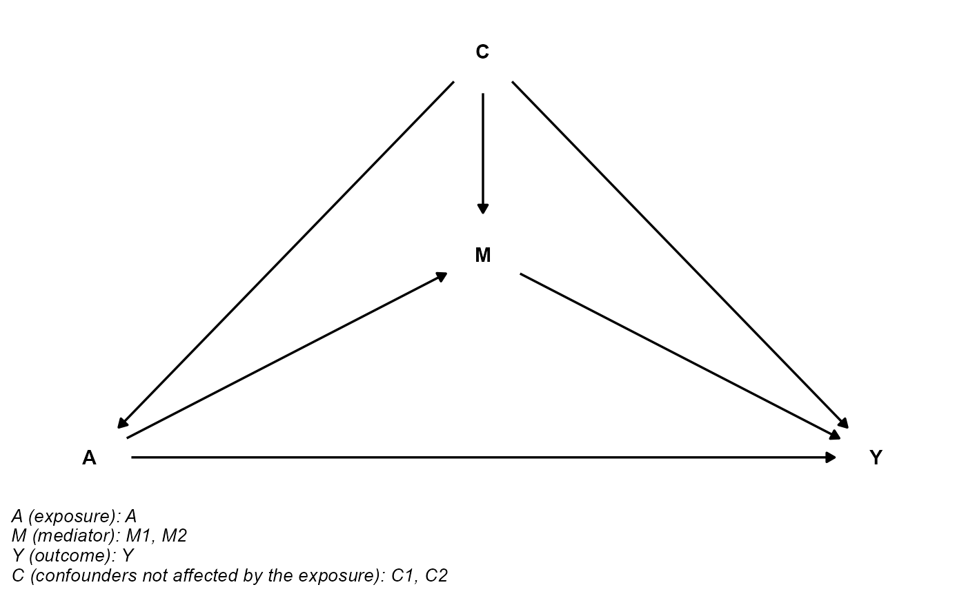
Then, we estimate causal effects using cmest. We use the
regression-based approach for illustration. The reference values for the
exposure are set to be 0 and 1. The reference values for the two
mediators are set to be 1.
est <- cmest(data = data, model = "rb", outcome = "Y", exposure = "A",
                mediator = c("M1", "M2"), basec = c("C1", "C2"), EMint = TRUE,
                mreg = list("logistic", "linear"), yreg = "linear",
                astar = 0, a = 1, mval = list(1, 1),
                estimation = "imputation", inference = "bootstrap", nboot = 20)
Summarize and plot the results:
summary(est)## Causal Mediation Analysis
##
## # Outcome regression:
##
## Call:
## glm(formula = Y ~ A + M1 + M2 + A * M1 + A * M2 + C1 + C2, family = gaussian(),
## data = getCall(x$reg.output$yreg)$data, weights = getCall(x$reg.output$yreg)$weights)
##
## Coefficients:
## Estimate Std. Error t value Pr(>|t|)
## (Intercept) -0.429317 0.446678 -0.961 0.3390
## A 1.305199 0.751816 1.736 0.0859 .
## M1 0.762169 0.310811 2.452 0.0161 *
## M2 0.691868 0.132038 5.240 1.01e-06 ***
## C1 -0.197350 0.136885 -1.442 0.1528
## C2 2.389790 0.355404 6.724 1.46e-09 ***
## A:M1 0.127853 0.466496 0.274 0.7846
## A:M2 -0.001608 0.151163 -0.011 0.9915
## ---
## Signif. codes: 0 '***' 0.001 '**' 0.01 '*' 0.05 '.' 0.1 ' ' 1
##
## (Dispersion parameter for gaussian family taken to be 1.100923)
##
## Null deviance: 571.51 on 99 degrees of freedom
## Residual deviance: 101.28 on 92 degrees of freedom
## AIC: 303.06
##
## Number of Fisher Scoring iterations: 2
##
##
## # Mediator regressions:
##
## Call:
## glm(formula = M1 ~ A + C1 + C2, family = binomial(), data = getCall(x$reg.output$mreg[[1L]])$data,
## weights = getCall(x$reg.output$mreg[[1L]])$weights)
##
## Coefficients:
## Estimate Std. Error z value Pr(>|z|)
## (Intercept) 0.003446 0.547959 0.006 0.994982
## A 0.828694 0.456732 1.814 0.069616 .
## C1 -0.984454 0.292880 -3.361 0.000776 ***
## C2 0.892199 0.511832 1.743 0.081308 .
## ---
## Signif. codes: 0 '***' 0.001 '**' 0.01 '*' 0.05 '.' 0.1 ' ' 1
##
## (Dispersion parameter for binomial family taken to be 1)
##
## Null deviance: 138.47 on 99 degrees of freedom
## Residual deviance: 115.67 on 96 degrees of freedom
## AIC: 123.67
##
## Number of Fisher Scoring iterations: 3
##
##
##
## Call:
## glm(formula = M2 ~ A + C1 + C2, family = gaussian(), data = getCall(x$reg.output$mreg[[2L]])$data,
## weights = getCall(x$reg.output$mreg[[2L]])$weights)
##
## Coefficients:
## Estimate Std. Error t value Pr(>|t|)
## (Intercept) 1.6403 0.2564 6.397 5.75e-09 ***
## A 0.2901 0.2170 1.337 0.184
## C1 0.6208 0.1189 5.219 1.04e-06 ***
## C2 2.0833 0.2366 8.806 5.44e-14 ***
## ---
## Signif. codes: 0 '***' 0.001 '**' 0.01 '*' 0.05 '.' 0.1 ' ' 1
##
## (Dispersion parameter for gaussian family taken to be 1.110528)
##
## Null deviance: 225.08 on 99 degrees of freedom
## Residual deviance: 106.61 on 96 degrees of freedom
## AIC: 300.19
##
## Number of Fisher Scoring iterations: 2
##
##
## # Effect decomposition on the mean difference scale via the regression-based approach
##
## Direct counterfactual imputation estimation with
## bootstrap standard errors, percentile confidence intervals and p-values
##
## Estimate Std.error 95% CIL 95% CIU P.val
## cde 1.431445 0.431151 0.589084 1.966 <2e-16 ***
## pnde 1.358006 0.258199 0.795697 1.671 <2e-16 ***
## tnde 1.370325 0.290368 0.937364 1.820 <2e-16 ***
## pnie 0.276953 0.193599 0.085562 0.698 <2e-16 ***
## tnie 0.289272 0.168953 0.218565 0.775 <2e-16 ***
## te 1.647278 0.234166 1.246535 2.056 <2e-16 ***
## intref -0.073439 0.356733 -0.595168 0.627 0.6
## intmed 0.012319 0.159298 -0.286255 0.212 0.9
## cde(prop) 0.868976 0.222221 0.390778 1.099 <2e-16 ***
## intref(prop) -0.044582 0.215448 -0.357290 0.378 0.6
## intmed(prop) 0.007478 0.093154 -0.155366 0.133 0.9
## pnie(prop) 0.168128 0.114003 0.052402 0.405 <2e-16 ***
## pm 0.175606 0.101672 0.135993 0.449 <2e-16 ***
## int -0.037103 0.201112 -0.374002 0.369 0.8
## pe 0.131024 0.222221 -0.098608 0.609 0.4
## ---
## Signif. codes: 0 '***' 0.001 '**' 0.01 '*' 0.05 '.' 0.1 ' ' 1
##
## (cde: controlled direct effect; pnde: pure natural direct effect; tnde: total natural direct effect; pnie: pure natural indirect effect; tnie: total natural indirect effect; te: total effect; intref: reference interaction; intmed: mediated interaction; cde(prop): proportion cde; intref(prop): proportion intref; intmed(prop): proportion intmed; pnie(prop): proportion pnie; pm: overall proportion mediated; int: overall proportion attributable to interaction; pe: overall proportion eliminated)
##
## Relevant variable values:
## $a
## [1] 1
##
## $astar
## [1] 0
##
## $mval
## $mval[[1]]
## [1] 1
##
## $mval[[2]]
## [1] 1
ggcmest(est) +
  ggplot2::theme(axis.text.x = ggplot2::element_text(angle = 30, vjust = 0.8))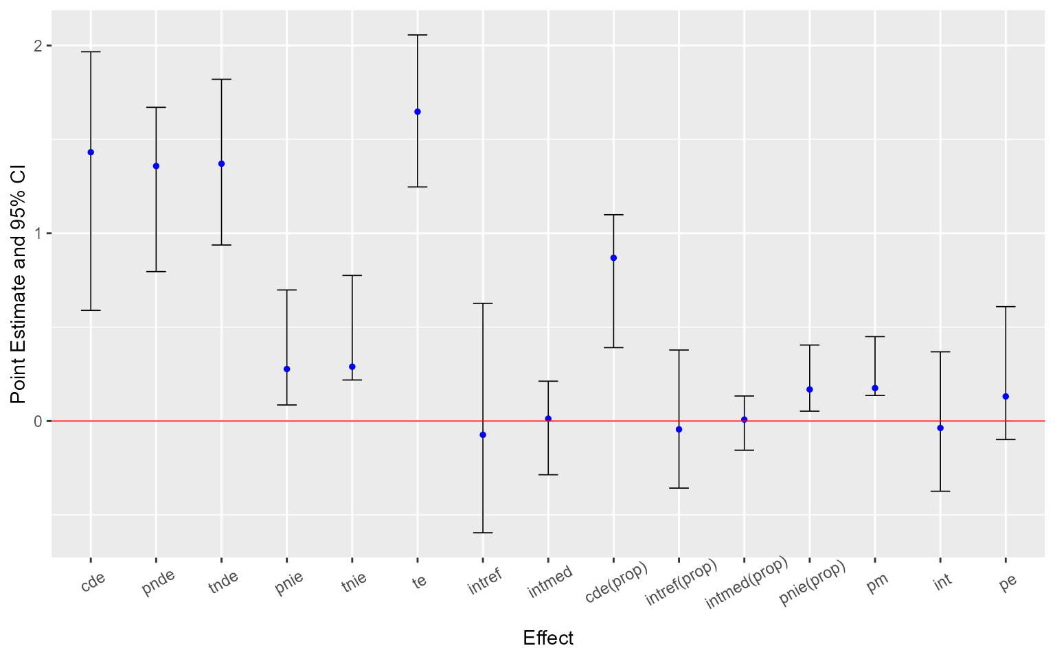
Lastly, we conduct sensitivity analysis for the results. Sensitivity analysis for unmeasured confounding:
cmsens(object = est, sens = "uc")## Sensitivity Analysis For Unmeasured Confounding
##
## Evalues on the risk or rate ratio scale:
## estRR lowerRR upperRR Evalue.estRR Evalue.lowerRR Evalue.upperRR
## cde 1.719704 1.2494926 2.366867 2.832214 1.807829 NA
## pnde 1.672531 1.3813387 2.025107 2.733110 2.107120 NA
## tnde 1.680352 1.3551158 2.083648 2.749573 2.048818 NA
## pnie 1.110593 0.9622016 1.281871 1.461057 1.000000 NA
## tnie 1.115787 0.9845137 1.264565 1.475223 1.000000 NA
## te 1.866188 1.5689678 2.219714 3.137593 2.513792 NAAssume that was measured with error. Sensitivity analysis for measurement error using regression calibration with a set of assumed error standard deviations 0.1, 0.2 and 0.3:
me1 <- cmsens(object = est, sens = "me", MEmethod = "rc",
              MEvariable = "C1", MEvartype = "con", MEerror = c(0.1, 0.2, 0.3))
Summarize and plot the results:
summary(me1)## Sensitivity Analysis For Measurement Error
##
## The variable measured with error: C1
## Type of the variable measured with error: continuous
##
## # Measurement error 1:
## [1] 0.1
##
## ## Error-corrected regressions for measurement error 1:
##
## ### Outcome regression:
## Call:
## rcreg(reg = getCall(x$sens[[1L]]$reg.output$yreg)$reg, formula = Y ~
## A + M1 + M2 + A * M1 + A * M2 + C1 + C2, data = getCall(x$sens[[1L]]$reg.output$yreg)$data,
## MEvariable = "C1", MEerror = 0.1, variance = TRUE, nboot = 400,
## weights = getCall(x$sens[[1L]]$reg.output$yreg)$weights)
##
## Naive coefficient estimates:
## (Intercept) A M1 M2 C1 C2
## -0.429317055 1.305199111 0.762169424 0.691868043 -0.197349688 2.389790272
## A:M1 A:M2
## 0.127853354 -0.001607689
##
## Naive var-cov estimates:
## (Intercept) A M1 M2 C1
## (Intercept) 0.19952129 -0.186177297 -0.071800151 -0.042143887 -0.012473494
## A -0.18617730 0.565227608 0.061763824 0.035566831 0.008550886
## M1 -0.07180015 0.061763824 0.096603550 0.011127995 0.008367323
## M2 -0.04214389 0.035566831 0.011127995 0.017433949 -0.005541985
## C1 -0.01247349 0.008550886 0.008367323 -0.005541985 0.018737581
## C2 0.03202116 -0.002076496 -0.025485517 -0.031937394 0.011413789
## A:M1 0.05250394 -0.194186113 -0.081844376 0.001218548 -0.006350845
## A:M2 0.03868322 -0.102112096 -0.008061219 -0.010381316 -0.000334026
## C2 A:M1 A:M2
## (Intercept) 0.032021156 0.052503937 0.038683218
## A -0.002076496 -0.194186113 -0.102112096
## M1 -0.025485517 -0.081844376 -0.008061219
## M2 -0.031937394 0.001218548 -0.010381316
## C1 0.011413789 -0.006350845 -0.000334026
## C2 0.126311866 -0.027375016 0.006147880
## A:M1 -0.027375016 0.217618968 0.019236723
## A:M2 0.006147880 0.019236723 0.022850334
##
## Variable measured with error:
## C1
## Measurement error:
## 0.1
## Error-corrected results:
## Estimate Std. Error t value Pr(>|t|)
## (Intercept) -0.427276 0.474476 -0.901 0.3702
## A 1.304514 0.686210 1.901 0.0604 .
## M1 0.761089 0.368519 2.065 0.0417 *
## M2 0.692841 0.131912 5.252 9.64e-07 ***
## C1 -0.200697 0.120068 -1.672 0.0980 .
## C2 2.387891 0.391831 6.094 2.54e-08 ***
## A:M1 0.127853 0.405801 0.315 0.7534
## A:M2 -0.001608 0.144675 -0.011 0.9912
## ---
## Signif. codes: 0 '***' 0.001 '**' 0.01 '*' 0.05 '.' 0.1 ' ' 1
##
## ### Mediator regressions:
## Call:
## rcreg(reg = getCall(x$sens[[1L]]$reg.output$mreg[[1L]])$reg,
## formula = M1 ~ A + C1 + C2, data = getCall(x$sens[[1L]]$reg.output$mreg[[1L]])$data,
## MEvariable = "C1", MEerror = 0.1, variance = TRUE, nboot = 400,
## weights = getCall(x$sens[[1L]]$reg.output$mreg[[1L]])$weights)
##
## Naive coefficient estimates:
## (Intercept) A C1 C2
## 0.003446339 0.828694328 -0.984453987 0.892199087
##
## Naive var-cov estimates:
## (Intercept) A C1 C2
## (Intercept) 0.30025921 -0.07438249 -0.08381839 -0.17194314
## A -0.07438249 0.20860406 -0.00266003 -0.01458923
## C1 -0.08381839 -0.00266003 0.08577848 -0.01275232
## C2 -0.17194314 -0.01458923 -0.01275232 0.26197192
##
## Variable measured with error:
## C1
## Measurement error:
## 0.1
## Error-corrected results:
## Estimate Std. Error t value Pr(>|t|)
## (Intercept) 0.01887 0.60385 0.031 0.9751
## A 0.82577 0.46685 1.769 0.0801 .
## C1 -0.99703 0.39058 -2.553 0.0123 *
## C2 0.89185 0.56574 1.576 0.1182
## ---
## Signif. codes: 0 '***' 0.001 '**' 0.01 '*' 0.05 '.' 0.1 ' ' 1
##
## Call:
## rcreg(reg = getCall(x$sens[[1L]]$reg.output$mreg[[2L]])$reg,
## formula = M2 ~ A + C1 + C2, data = getCall(x$sens[[1L]]$reg.output$mreg[[2L]])$data,
## MEvariable = "C1", MEerror = 0.1, variance = TRUE, nboot = 400,
## weights = getCall(x$sens[[1L]]$reg.output$mreg[[2L]])$weights)
##
## Naive coefficient estimates:
## (Intercept) A C1 C2
## 1.6402566 0.2901364 0.6208107 2.0833115
##
## Naive var-cov estimates:
## (Intercept) A C1 C2
## (Intercept) 0.06573913 -0.018924346 -0.0173562931 -0.0381103530
## A -0.01892435 0.047073002 0.0032931500 -0.0062472874
## C1 -0.01735629 0.003293150 0.0141472682 0.0003964488
## C2 -0.03811035 -0.006247287 0.0003964488 0.0559647177
##
## Variable measured with error:
## C1
## Measurement error:
## 0.2
## Error-corrected results:
## Estimate Std. Error t value Pr(>|t|)
## (Intercept) 1.5998 0.2376 6.732 1.22e-09 ***
## A 0.2978 0.2121 1.404 0.164
## C1 0.6538 0.1414 4.624 1.18e-05 ***
## C2 2.0842 0.1865 11.175 < 2e-16 ***
## ---
## Signif. codes: 0 '***' 0.001 '**' 0.01 '*' 0.05 '.' 0.1 ' ' 1
##
##
## ## Error-corrected causal effects on the mean difference scale for measurement error 1:
## Estimate Std.error 95% CIL 95% CIU P.val
## cde 1.43076 0.50986 0.49889 2.224 <2e-16 ***
## pnde 1.34565 0.16116 1.13735 1.694 <2e-16 ***
## tnde 1.37203 0.16903 1.12925 1.692 <2e-16 ***
## pnie 0.36213 0.17977 -0.04486 0.637 0.1 .
## tnie 0.38851 0.14743 0.01110 0.560 0.1 .
## te 1.73416 0.19016 1.37939 2.058 <2e-16 ***
## intref -0.08511 0.48639 -0.75376 0.859 0.7
## intmed 0.02638 0.11009 -0.13662 0.228 0.7
## cde(prop) 0.82505 0.27223 0.31807 1.275 <2e-16 ***
## intref(prop) -0.04908 0.29125 -0.43234 0.527 0.7
## intmed(prop) 0.01521 0.06418 -0.07733 0.138 0.7
## pnie(prop) 0.20882 0.10187 -0.03697 0.360 0.1 .
## pm 0.22403 0.08676 0.00266 0.319 0.1 .
## int -0.03386 0.28825 -0.41072 0.571 0.8
## pe 0.17495 0.27223 -0.27496 0.682 0.3
## ---
## Signif. codes: 0 '***' 0.001 '**' 0.01 '*' 0.05 '.' 0.1 ' ' 1
## ----------------------------------------------------------------
##
## # Measurement error 2:
## [1] 0.2
##
## ## Error-corrected regressions for measurement error 2:
##
## ### Outcome regression:
## Call:
## rcreg(reg = getCall(x$sens[[2L]]$reg.output$yreg)$reg, formula = Y ~
## A + M1 + M2 + A * M1 + A * M2 + C1 + C2, data = getCall(x$sens[[2L]]$reg.output$yreg)$data,
## MEvariable = "C1", MEerror = 0.2, variance = TRUE, nboot = 400,
## weights = getCall(x$sens[[2L]]$reg.output$yreg)$weights)
##
## Naive coefficient estimates:
## (Intercept) A M1 M2 C1 C2
## -0.429317055 1.305199111 0.762169424 0.691868043 -0.197349688 2.389790272
## A:M1 A:M2
## 0.127853354 -0.001607689
##
## Naive var-cov estimates:
## (Intercept) A M1 M2 C1
## (Intercept) 0.19952129 -0.186177297 -0.071800151 -0.042143887 -0.012473494
## A -0.18617730 0.565227608 0.061763824 0.035566831 0.008550886
## M1 -0.07180015 0.061763824 0.096603550 0.011127995 0.008367323
## M2 -0.04214389 0.035566831 0.011127995 0.017433949 -0.005541985
## C1 -0.01247349 0.008550886 0.008367323 -0.005541985 0.018737581
## C2 0.03202116 -0.002076496 -0.025485517 -0.031937394 0.011413789
## A:M1 0.05250394 -0.194186113 -0.081844376 0.001218548 -0.006350845
## A:M2 0.03868322 -0.102112096 -0.008061219 -0.010381316 -0.000334026
## C2 A:M1 A:M2
## (Intercept) 0.032021156 0.052503937 0.038683218
## A -0.002076496 -0.194186113 -0.102112096
## M1 -0.025485517 -0.081844376 -0.008061219
## M2 -0.031937394 0.001218548 -0.010381316
## C1 0.011413789 -0.006350845 -0.000334026
## C2 0.126311866 -0.027375016 0.006147880
## A:M1 -0.027375016 0.217618968 0.019236723
## A:M2 0.006147880 0.019236723 0.022850334
##
## Variable measured with error:
## C1
## Measurement error:
## 0.2
## Error-corrected results:
## Estimate Std. Error t value Pr(>|t|)
## (Intercept) -0.420717 0.446142 -0.943 0.3481
## A 1.302311 0.705424 1.846 0.0681 .
## M1 0.757615 0.346468 2.187 0.0313 *
## M2 0.695971 0.138808 5.014 2.58e-06 ***
## C1 -0.211459 0.130027 -1.626 0.1073
## C2 2.381786 0.418420 5.692 1.48e-07 ***
## A:M1 0.127853 0.413179 0.309 0.7577
## A:M2 -0.001608 0.148853 -0.011 0.9914
## ---
## Signif. codes: 0 '***' 0.001 '**' 0.01 '*' 0.05 '.' 0.1 ' ' 1
##
## ### Mediator regressions:
## Call:
## rcreg(reg = getCall(x$sens[[2L]]$reg.output$mreg[[1L]])$reg,
## formula = M1 ~ A + C1 + C2, data = getCall(x$sens[[2L]]$reg.output$mreg[[1L]])$data,
## MEvariable = "C1", MEerror = 0.2, variance = TRUE, nboot = 400,
## weights = getCall(x$sens[[2L]]$reg.output$mreg[[1L]])$weights)
##
## Naive coefficient estimates:
## (Intercept) A C1 C2
## 0.003446339 0.828694328 -0.984453987 0.892199087
##
## Naive var-cov estimates:
## (Intercept) A C1 C2
## (Intercept) 0.30025921 -0.07438249 -0.08381839 -0.17194314
## A -0.07438249 0.20860406 -0.00266003 -0.01458923
## C1 -0.08381839 -0.00266003 0.08577848 -0.01275232
## C2 -0.17194314 -0.01458923 -0.01275232 0.26197192
##
## Variable measured with error:
## C1
## Measurement error:
## 0.1
## Error-corrected results:
## Estimate Std. Error t value Pr(>|t|)
## (Intercept) 0.01887 0.60385 0.031 0.9751
## A 0.82577 0.46685 1.769 0.0801 .
## C1 -0.99703 0.39058 -2.553 0.0123 *
## C2 0.89185 0.56574 1.576 0.1182
## ---
## Signif. codes: 0 '***' 0.001 '**' 0.01 '*' 0.05 '.' 0.1 ' ' 1
##
## Call:
## rcreg(reg = getCall(x$sens[[2L]]$reg.output$mreg[[2L]])$reg,
## formula = M2 ~ A + C1 + C2, data = getCall(x$sens[[2L]]$reg.output$mreg[[2L]])$data,
## MEvariable = "C1", MEerror = 0.2, variance = TRUE, nboot = 400,
## weights = getCall(x$sens[[2L]]$reg.output$mreg[[2L]])$weights)
##
## Naive coefficient estimates:
## (Intercept) A C1 C2
## 1.6402566 0.2901364 0.6208107 2.0833115
##
## Naive var-cov estimates:
## (Intercept) A C1 C2
## (Intercept) 0.06573913 -0.018924346 -0.0173562931 -0.0381103530
## A -0.01892435 0.047073002 0.0032931500 -0.0062472874
## C1 -0.01735629 0.003293150 0.0141472682 0.0003964488
## C2 -0.03811035 -0.006247287 0.0003964488 0.0559647177
##
## Variable measured with error:
## C1
## Measurement error:
## 0.2
## Error-corrected results:
## Estimate Std. Error t value Pr(>|t|)
## (Intercept) 1.5998 0.2376 6.732 1.22e-09 ***
## A 0.2978 0.2121 1.404 0.164
## C1 0.6538 0.1414 4.624 1.18e-05 ***
## C2 2.0842 0.1865 11.175 < 2e-16 ***
## ---
## Signif. codes: 0 '***' 0.001 '**' 0.01 '*' 0.05 '.' 0.1 ' ' 1
##
##
## ## Error-corrected causal effects on the mean difference scale for measurement error 2:
## Estimate Std.error 95% CIL 95% CIU P.val
## cde 1.428557 0.669836 0.244304 2.548 <2e-16 ***
## pnde 1.356446 0.215239 1.156362 1.761 <2e-16 ***
## tnde 1.366196 0.202015 1.173299 1.831 <2e-16 ***
## pnie 0.267879 0.135532 0.059300 0.558 0.1 .
## tnie 0.277628 0.121579 0.033675 0.503 0.1 .
## te 1.634074 0.250486 1.247528 2.111 <2e-16 ***
## intref -0.072111 0.575551 -0.864093 1.037 0.7
## intmed 0.009749 0.095543 -0.204712 0.105 0.7
## cde(prop) 0.874230 0.373296 0.148454 1.406 <2e-16 ***
## intref(prop) -0.044129 0.342897 -0.513162 0.651 0.7
## intmed(prop) 0.005966 0.050230 -0.099077 0.057 0.7
## pnie(prop) 0.163933 0.068998 0.029984 0.272 0.1 .
## pm 0.169899 0.067892 0.017890 0.281 0.1 .
## int -0.038163 0.369741 -0.523288 0.707 0.8
## pe 0.125770 0.373296 -0.405694 0.852 0.9
## ---
## Signif. codes: 0 '***' 0.001 '**' 0.01 '*' 0.05 '.' 0.1 ' ' 1
## ----------------------------------------------------------------
##
## # Measurement error 3:
## [1] 0.3
##
## ## Error-corrected regressions for measurement error 3:
##
## ### Outcome regression:
## Call:
## rcreg(reg = getCall(x$sens[[3L]]$reg.output$yreg)$reg, formula = Y ~
## A + M1 + M2 + A * M1 + A * M2 + C1 + C2, data = getCall(x$sens[[3L]]$reg.output$yreg)$data,
## MEvariable = "C1", MEerror = 0.3, variance = TRUE, nboot = 400,
## weights = getCall(x$sens[[3L]]$reg.output$yreg)$weights)
##
## Naive coefficient estimates:
## (Intercept) A M1 M2 C1 C2
## -0.429317055 1.305199111 0.762169424 0.691868043 -0.197349688 2.389790272
## A:M1 A:M2
## 0.127853354 -0.001607689
##
## Naive var-cov estimates:
## (Intercept) A M1 M2 C1
## (Intercept) 0.19952129 -0.186177297 -0.071800151 -0.042143887 -0.012473494
## A -0.18617730 0.565227608 0.061763824 0.035566831 0.008550886
## M1 -0.07180015 0.061763824 0.096603550 0.011127995 0.008367323
## M2 -0.04214389 0.035566831 0.011127995 0.017433949 -0.005541985
## C1 -0.01247349 0.008550886 0.008367323 -0.005541985 0.018737581
## C2 0.03202116 -0.002076496 -0.025485517 -0.031937394 0.011413789
## A:M1 0.05250394 -0.194186113 -0.081844376 0.001218548 -0.006350845
## A:M2 0.03868322 -0.102112096 -0.008061219 -0.010381316 -0.000334026
## C2 A:M1 A:M2
## (Intercept) 0.032021156 0.052503937 0.038683218
## A -0.002076496 -0.194186113 -0.102112096
## M1 -0.025485517 -0.081844376 -0.008061219
## M2 -0.031937394 0.001218548 -0.010381316
## C1 0.011413789 -0.006350845 -0.000334026
## C2 0.126311866 -0.027375016 0.006147880
## A:M1 -0.027375016 0.217618968 0.019236723
## A:M2 0.006147880 0.019236723 0.022850334
##
## Variable measured with error:
## C1
## Measurement error:
## 0.3
## Error-corrected results:
## Estimate Std. Error t value Pr(>|t|)
## (Intercept) -0.408067 0.467151 -0.874 0.3847
## A 1.298063 0.804716 1.613 0.1102
## M1 0.750917 0.359096 2.091 0.0393 *
## M2 0.702005 0.151218 4.642 1.14e-05 ***
## C1 -0.232211 0.160485 -1.447 0.1513
## C2 2.370014 0.389950 6.078 2.73e-08 ***
## A:M1 0.127853 0.428765 0.298 0.7662
## A:M2 -0.001608 0.167286 -0.010 0.9924
## ---
## Signif. codes: 0 '***' 0.001 '**' 0.01 '*' 0.05 '.' 0.1 ' ' 1
##
## ### Mediator regressions:
## Call:
## rcreg(reg = getCall(x$sens[[3L]]$reg.output$mreg[[1L]])$reg,
## formula = M1 ~ A + C1 + C2, data = getCall(x$sens[[3L]]$reg.output$mreg[[1L]])$data,
## MEvariable = "C1", MEerror = 0.3, variance = TRUE, nboot = 400,
## weights = getCall(x$sens[[3L]]$reg.output$mreg[[1L]])$weights)
##
## Naive coefficient estimates:
## (Intercept) A C1 C2
## 0.003446339 0.828694328 -0.984453987 0.892199087
##
## Naive var-cov estimates:
## (Intercept) A C1 C2
## (Intercept) 0.30025921 -0.07438249 -0.08381839 -0.17194314
## A -0.07438249 0.20860406 -0.00266003 -0.01458923
## C1 -0.08381839 -0.00266003 0.08577848 -0.01275232
## C2 -0.17194314 -0.01458923 -0.01275232 0.26197192
##
## Variable measured with error:
## C1
## Measurement error:
## 0.1
## Error-corrected results:
## Estimate Std. Error t value Pr(>|t|)
## (Intercept) 0.01887 0.60385 0.031 0.9751
## A 0.82577 0.46685 1.769 0.0801 .
## C1 -0.99703 0.39058 -2.553 0.0123 *
## C2 0.89185 0.56574 1.576 0.1182
## ---
## Signif. codes: 0 '***' 0.001 '**' 0.01 '*' 0.05 '.' 0.1 ' ' 1
##
## Call:
## rcreg(reg = getCall(x$sens[[3L]]$reg.output$mreg[[2L]])$reg,
## formula = M2 ~ A + C1 + C2, data = getCall(x$sens[[3L]]$reg.output$mreg[[2L]])$data,
## MEvariable = "C1", MEerror = 0.3, variance = TRUE, nboot = 400,
## weights = getCall(x$sens[[3L]]$reg.output$mreg[[2L]])$weights)
##
## Naive coefficient estimates:
## (Intercept) A C1 C2
## 1.6402566 0.2901364 0.6208107 2.0833115
##
## Naive var-cov estimates:
## (Intercept) A C1 C2
## (Intercept) 0.06573913 -0.018924346 -0.0173562931 -0.0381103530
## A -0.01892435 0.047073002 0.0032931500 -0.0062472874
## C1 -0.01735629 0.003293150 0.0141472682 0.0003964488
## C2 -0.03811035 -0.006247287 0.0003964488 0.0559647177
##
## Variable measured with error:
## C1
## Measurement error:
## 0.2
## Error-corrected results:
## Estimate Std. Error t value Pr(>|t|)
## (Intercept) 1.5998 0.2376 6.732 1.22e-09 ***
## A 0.2978 0.2121 1.404 0.164
## C1 0.6538 0.1414 4.624 1.18e-05 ***
## C2 2.0842 0.1865 11.175 < 2e-16 ***
## ---
## Signif. codes: 0 '***' 0.001 '**' 0.01 '*' 0.05 '.' 0.1 ' ' 1
##
##
## ## Error-corrected causal effects on the mean difference scale for measurement error 3:
## Estimate Std.error 95% CIL 95% CIU P.val
## cde 1.42431 0.46307 0.61956 2.175 <2e-16 ***
## pnde 1.33804 0.22658 1.02865 1.815 <2e-16 ***
## tnde 1.36311 0.22654 0.99180 1.763 <2e-16 ***
## pnie 0.36685 0.20087 0.01872 0.733 0.1 .
## tnie 0.39192 0.15468 0.04867 0.621 0.1 .
## te 1.72996 0.27424 1.21911 2.190 <2e-16 ***
## intref -0.08627 0.37031 -0.69366 0.529 0.8
## intmed 0.02507 0.10160 -0.23636 0.129 0.9
## cde(prop) 0.82332 0.21876 0.48183 1.191 <2e-16 ***
## intref(prop) -0.04987 0.23370 -0.38643 0.380 0.8
## intmed(prop) 0.01449 0.05573 -0.12205 0.077 0.9
## pnie(prop) 0.21206 0.10239 0.01209 0.395 0.1 .
## pm 0.22655 0.07850 0.02840 0.330 0.1 .
## int -0.03538 0.24894 -0.44175 0.392 0.8
## pe 0.17668 0.21876 -0.19142 0.518 0.5
## ---
## Signif. codes: 0 '***' 0.001 '**' 0.01 '*' 0.05 '.' 0.1 ' ' 1
## ----------------------------------------------------------------
##
## (cde: controlled direct effect; pnde: pure natural direct effect; tnde: total natural direct effect; pnie: pure natural indirect effect; tnie: total natural indirect effect; te: total effect; intref: reference interaction; intmed: mediated interaction; cde(prop): proportion cde; intref(prop): proportion intref; intmed(prop): proportion intmed; pnie(prop): proportion pnie; pm: overall proportion mediated; int: overall proportion attributable to interaction; pe: overall proportion eliminated)
##
## Relevant variable values:
## $a
## [1] 1
##
## $astar
## [1] 0
##
## $mval
## $mval[[1]]
## [1] 1
##
## $mval[[2]]
## [1] 1
ggcmsens(me1) +
  ggplot2::theme(axis.text.x = ggplot2::element_text(angle = 30, vjust = 0.8))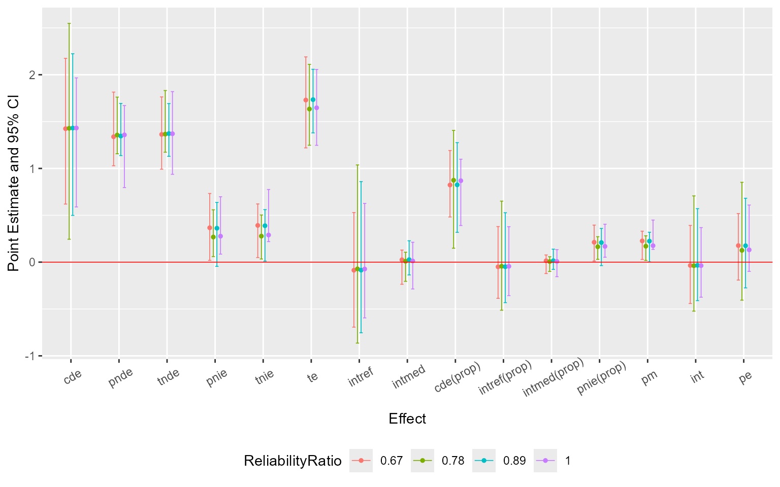
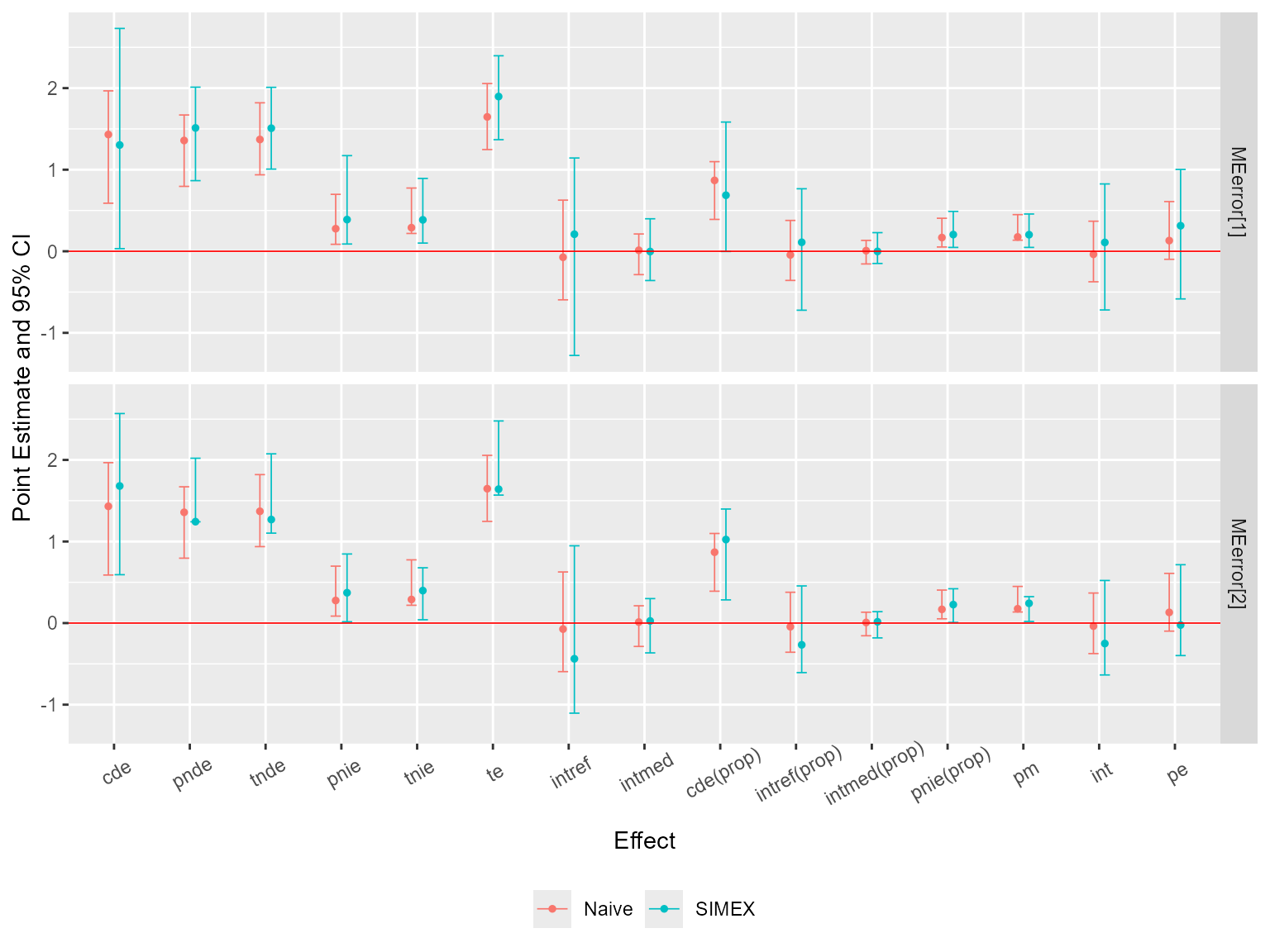
Then, assume that the exposure was measured with error. Sensitivity analysis for measurement error using SIMEX with two assumed misclassification matrices:
me2 <- cmsens(object = est, sens = "me", MEmethod = "simex", MEvariable = "A",
              MEvartype = "cat", B = 5,
              MEerror = list(matrix(c(0.95, 0.05, 0.05, 0.95), nrow = 2),
                             matrix(c(0.9, 0.1, 0.1, 0.9), nrow = 2)))
Summarize and plot the results:
summary(me2)## Sensitivity Analysis For Measurement Error
##
## The variable measured with error: A
## Type of the variable measured with error: categorical
##
## # Measurement error 1:
## [,1] [,2]
## [1,] 0.95 0.05
## [2,] 0.05 0.95
##
## ## Error-corrected regressions for measurement error 1:
##
## ### Outcome regression:
## Call:
## simexreg(reg = getCall(x$sens[[1L]]$reg.output$yreg)$reg, formula = Y ~
## A + M1 + M2 + A * M1 + A * M2 + C1 + C2, data = getCall(x$sens[[1L]]$reg.output$yreg)$data,
## MEvariable = "A", MEvartype = "categorical", MEerror = c(0.95,
## 0.05, 0.05, 0.95), variance = TRUE, lambda = c(0.5, 1, 1.5,
## 2), B = 5, weights = getCall(x$sens[[1L]]$reg.output$yreg)$weights)
##
## Naive coefficient estimates:
## (Intercept) A M1 M2 C1 C2
## -0.429317055 1.305199111 0.762169424 0.691868043 -0.197349688 2.389790272
## A:M1 A:M2
## 0.127853354 -0.001607689
##
## Naive var-cov estimates:
## (Intercept) A M1 M2 C1
## (Intercept) 0.19952129 -0.186177297 -0.071800151 -0.042143887 -0.012473494
## A -0.18617730 0.565227608 0.061763824 0.035566831 0.008550886
## M1 -0.07180015 0.061763824 0.096603550 0.011127995 0.008367323
## M2 -0.04214389 0.035566831 0.011127995 0.017433949 -0.005541985
## C1 -0.01247349 0.008550886 0.008367323 -0.005541985 0.018737581
## C2 0.03202116 -0.002076496 -0.025485517 -0.031937394 0.011413789
## A:M1 0.05250394 -0.194186113 -0.081844376 0.001218548 -0.006350845
## A:M2 0.03868322 -0.102112096 -0.008061219 -0.010381316 -0.000334026
## C2 A:M1 A:M2
## (Intercept) 0.032021156 0.052503937 0.038683218
## A -0.002076496 -0.194186113 -0.102112096
## M1 -0.025485517 -0.081844376 -0.008061219
## M2 -0.031937394 0.001218548 -0.010381316
## C1 0.011413789 -0.006350845 -0.000334026
## C2 0.126311866 -0.027375016 0.006147880
## A:M1 -0.027375016 0.217618968 0.019236723
## A:M2 0.006147880 0.019236723 0.022850334
##
## Variable measured with error:
## A
## Measurement error:
## 0 1
## 0 0.95 0.05
## 1 0.05 0.95
##
## Error-corrected results:
## Estimate Std. Error t value Pr(>|t|)
## (Intercept) -0.37768 0.47543 -0.794 0.42902
## A 1.33134 0.63147 2.108 0.03772 *
## M1 0.78640 0.24872 3.162 0.00212 **
## M2 0.65456 0.12916 5.068 2.07e-06 ***
## C1 -0.17222 0.14706 -1.171 0.24459
## C2 2.41490 0.34130 7.076 2.87e-10 ***
## A:M1 -0.08382 0.31928 -0.263 0.79350
## A:M2 0.05523 0.11903 0.464 0.64375
## ---
## Signif. codes: 0 '***' 0.001 '**' 0.01 '*' 0.05 '.' 0.1 ' ' 1
##
## ### Mediator regressions:
## Call:
## simexreg(reg = getCall(x$sens[[1L]]$reg.output$mreg[[1L]])$reg,
## formula = M1 ~ A + C1 + C2, data = getCall(x$sens[[1L]]$reg.output$mreg[[1L]])$data,
## MEvariable = "A", MEvartype = "categorical", MEerror = c(0.95,
## 0.05, 0.05, 0.95), variance = TRUE, lambda = c(0.5, 1, 1.5,
## 2), B = 5, weights = getCall(x$sens[[1L]]$reg.output$mreg[[1L]])$weights)
##
## Naive coefficient estimates:
## (Intercept) A C1 C2
## 0.003446339 0.828694328 -0.984453987 0.892199087
##
## Naive var-cov estimates:
## (Intercept) A C1 C2
## (Intercept) 0.30025921 -0.07438249 -0.08381839 -0.17194314
## A -0.07438249 0.20860406 -0.00266003 -0.01458923
## C1 -0.08381839 -0.00266003 0.08577848 -0.01275232
## C2 -0.17194314 -0.01458923 -0.01275232 0.26197192
##
## Variable measured with error:
## A
## Measurement error:
## 0 1
## 0 0.95 0.05
## 1 0.05 0.95
##
## Error-corrected results:
## Estimate Std. Error t value Pr(>|t|)
## (Intercept) 0.06506 0.55294 0.118 0.90659
## A1 0.65701 0.47346 1.388 0.16844
## C1 -0.92514 0.29214 -3.167 0.00207 **
## C2 0.82945 0.50631 1.638 0.10465
## ---
## Signif. codes: 0 '***' 0.001 '**' 0.01 '*' 0.05 '.' 0.1 ' ' 1
##
## Call:
## simexreg(reg = getCall(x$sens[[1L]]$reg.output$mreg[[2L]])$reg,
## formula = M2 ~ A + C1 + C2, data = getCall(x$sens[[1L]]$reg.output$mreg[[2L]])$data,
## MEvariable = "A", MEvartype = "categorical", MEerror = c(0.95,
## 0.05, 0.05, 0.95), variance = TRUE, lambda = c(0.5, 1, 1.5,
## 2), B = 5, weights = getCall(x$sens[[1L]]$reg.output$mreg[[2L]])$weights)
##
## Naive coefficient estimates:
## (Intercept) A C1 C2
## 1.6402566 0.2901364 0.6208107 2.0833115
##
## Naive var-cov estimates:
## (Intercept) A C1 C2
## (Intercept) 0.06573913 -0.018924346 -0.0173562931 -0.0381103530
## A -0.01892435 0.047073002 0.0032931500 -0.0062472874
## C1 -0.01735629 0.003293150 0.0141472682 0.0003964488
## C2 -0.03811035 -0.006247287 0.0003964488 0.0559647177
##
## Variable measured with error:
## A
## Measurement error:
## 0 1
## 0 0.9 0.1
## 1 0.1 0.9
##
## Error-corrected results:
## Estimate Std. Error t value Pr(>|t|)
## (Intercept) 1.6513 0.2526 6.536 3.04e-09 ***
## A 0.3958 0.2565 1.543 0.126
## C1 0.6180 0.1199 5.155 1.36e-06 ***
## C2 2.0269 0.2421 8.372 4.62e-13 ***
## ---
## Signif. codes: 0 '***' 0.001 '**' 0.01 '*' 0.05 '.' 0.1 ' ' 1
##
##
## ## Error-corrected causal effects on the mean difference scale for measurement error 1:
## Estimate Std.error 95% CIL 95% CIU P.val
## cde 1.302752 0.848516 0.032234 2.732 0.1 .
## pnde 1.511722 0.319366 0.865659 2.011 <2e-16 ***
## tnde 1.508457 0.293794 1.007221 2.009 <2e-16 ***
## pnie 0.388453 0.321018 0.088980 1.172 <2e-16 ***
## tnie 0.385188 0.231557 0.100461 0.893 <2e-16 ***
## te 1.896910 0.325833 1.367759 2.397 <2e-16 ***
## intref 0.208971 0.769005 -1.277145 1.143 0.7
## intmed -0.003266 0.201521 -0.358530 0.398 0.8
## cde(prop) 0.686776 0.452914 -0.002818 1.584 0.1 .
## intref(prop) 0.110164 0.456050 -0.722538 0.766 0.7
## intmed(prop) -0.001722 0.105670 -0.149573 0.228 0.8
## pnie(prop) 0.204782 0.132151 0.047280 0.489 <2e-16 ***
## pm 0.203061 0.111103 0.047540 0.457 <2e-16 ***
## int 0.108442 0.473111 -0.719296 0.825 0.8
## pe 0.313224 0.452914 -0.583927 1.003 0.4
## ---
## Signif. codes: 0 '***' 0.001 '**' 0.01 '*' 0.05 '.' 0.1 ' ' 1
## ----------------------------------------------------------------
##
## # Measurement error 2:
## [,1] [,2]
## [1,] 0.9 0.1
## [2,] 0.1 0.9
##
## ## Error-corrected regressions for measurement error 2:
##
## ### Outcome regression:
## Call:
## simexreg(reg = getCall(x$sens[[2L]]$reg.output$yreg)$reg, formula = Y ~
## A + M1 + M2 + A * M1 + A * M2 + C1 + C2, data = getCall(x$sens[[2L]]$reg.output$yreg)$data,
## MEvariable = "A", MEvartype = "categorical", MEerror = c(0.9,
## 0.1, 0.1, 0.9), variance = TRUE, lambda = c(0.5, 1, 1.5,
## 2), B = 5, weights = getCall(x$sens[[2L]]$reg.output$yreg)$weights)
##
## Naive coefficient estimates:
## (Intercept) A M1 M2 C1 C2
## -0.429317055 1.305199111 0.762169424 0.691868043 -0.197349688 2.389790272
## A:M1 A:M2
## 0.127853354 -0.001607689
##
## Naive var-cov estimates:
## (Intercept) A M1 M2 C1
## (Intercept) 0.19952129 -0.186177297 -0.071800151 -0.042143887 -0.012473494
## A -0.18617730 0.565227608 0.061763824 0.035566831 0.008550886
## M1 -0.07180015 0.061763824 0.096603550 0.011127995 0.008367323
## M2 -0.04214389 0.035566831 0.011127995 0.017433949 -0.005541985
## C1 -0.01247349 0.008550886 0.008367323 -0.005541985 0.018737581
## C2 0.03202116 -0.002076496 -0.025485517 -0.031937394 0.011413789
## A:M1 0.05250394 -0.194186113 -0.081844376 0.001218548 -0.006350845
## A:M2 0.03868322 -0.102112096 -0.008061219 -0.010381316 -0.000334026
## C2 A:M1 A:M2
## (Intercept) 0.032021156 0.052503937 0.038683218
## A -0.002076496 -0.194186113 -0.102112096
## M1 -0.025485517 -0.081844376 -0.008061219
## M2 -0.031937394 0.001218548 -0.010381316
## C1 0.011413789 -0.006350845 -0.000334026
## C2 0.126311866 -0.027375016 0.006147880
## A:M1 -0.027375016 0.217618968 0.019236723
## A:M2 0.006147880 0.019236723 0.022850334
##
## Variable measured with error:
## A
## Measurement error:
## 0 1
## 0 0.9 0.1
## 1 0.1 0.9
##
## Error-corrected results:
## Estimate Std. Error t value Pr(>|t|)
## (Intercept) -0.30285 0.50263 -0.603 0.5483
## A 1.33783 0.84799 1.578 0.1181
## M1 0.67409 NaN NaN NaN
## M2 0.71846 0.16617 4.324 3.88e-05 ***
## C1 -0.27034 0.14318 -1.888 0.0622 .
## C2 2.34290 0.42130 5.561 2.61e-07 ***
## A:M1 0.41221 NaN NaN NaN
## A:M2 -0.06952 0.16569 -0.420 0.6758
## ---
## Signif. codes: 0 '***' 0.001 '**' 0.01 '*' 0.05 '.' 0.1 ' ' 1
##
## ### Mediator regressions:
## Call:
## simexreg(reg = getCall(x$sens[[2L]]$reg.output$mreg[[1L]])$reg,
## formula = M1 ~ A + C1 + C2, data = getCall(x$sens[[2L]]$reg.output$mreg[[1L]])$data,
## MEvariable = "A", MEvartype = "categorical", MEerror = c(0.9,
## 0.1, 0.1, 0.9), variance = TRUE, lambda = c(0.5, 1, 1.5,
## 2), B = 5, weights = getCall(x$sens[[2L]]$reg.output$mreg[[1L]])$weights)
##
## Naive coefficient estimates:
## (Intercept) A C1 C2
## 0.003446339 0.828694328 -0.984453987 0.892199087
##
## Naive var-cov estimates:
## (Intercept) A C1 C2
## (Intercept) 0.30025921 -0.07438249 -0.08381839 -0.17194314
## A -0.07438249 0.20860406 -0.00266003 -0.01458923
## C1 -0.08381839 -0.00266003 0.08577848 -0.01275232
## C2 -0.17194314 -0.01458923 -0.01275232 0.26197192
##
## Variable measured with error:
## A
## Measurement error:
## 0 1
## 0 0.95 0.05
## 1 0.05 0.95
##
## Error-corrected results:
## Estimate Std. Error t value Pr(>|t|)
## (Intercept) 0.06506 0.55294 0.118 0.90659
## A1 0.65701 0.47346 1.388 0.16844
## C1 -0.92514 0.29214 -3.167 0.00207 **
## C2 0.82945 0.50631 1.638 0.10465
## ---
## Signif. codes: 0 '***' 0.001 '**' 0.01 '*' 0.05 '.' 0.1 ' ' 1
##
## Call:
## simexreg(reg = getCall(x$sens[[2L]]$reg.output$mreg[[2L]])$reg,
## formula = M2 ~ A + C1 + C2, data = getCall(x$sens[[2L]]$reg.output$mreg[[2L]])$data,
## MEvariable = "A", MEvartype = "categorical", MEerror = c(0.9,
## 0.1, 0.1, 0.9), variance = TRUE, lambda = c(0.5, 1, 1.5,
## 2), B = 5, weights = getCall(x$sens[[2L]]$reg.output$mreg[[2L]])$weights)
##
## Naive coefficient estimates:
## (Intercept) A C1 C2
## 1.6402566 0.2901364 0.6208107 2.0833115
##
## Naive var-cov estimates:
## (Intercept) A C1 C2
## (Intercept) 0.06573913 -0.018924346 -0.0173562931 -0.0381103530
## A -0.01892435 0.047073002 0.0032931500 -0.0062472874
## C1 -0.01735629 0.003293150 0.0141472682 0.0003964488
## C2 -0.03811035 -0.006247287 0.0003964488 0.0559647177
##
## Variable measured with error:
## A
## Measurement error:
## 0 1
## 0 0.9 0.1
## 1 0.1 0.9
##
## Error-corrected results:
## Estimate Std. Error t value Pr(>|t|)
## (Intercept) 1.6513 0.2526 6.536 3.04e-09 ***
## A 0.3958 0.2565 1.543 0.126
## C1 0.6180 0.1199 5.155 1.36e-06 ***
## C2 2.0269 0.2421 8.372 4.62e-13 ***
## ---
## Signif. codes: 0 '***' 0.001 '**' 0.01 '*' 0.05 '.' 0.1 ' ' 1
##
##
## ## Error-corrected causal effects on the mean difference scale for measurement error 2:
## Estimate Std.error 95% CIL 95% CIU P.val
## cde 1.680525 0.553907 0.593068 2.569 <2e-16 ***
## pnde 1.243251 0.277715 1.241656 2.021 <2e-16 ***
## tnde 1.269322 0.337197 1.102621 2.075 <2e-16 ***
## pnie 0.372015 0.236894 0.016540 0.847 <2e-16 ***
## tnie 0.398086 0.190160 0.040929 0.678 <2e-16 ***
## te 1.641337 0.273621 1.568937 2.478 <2e-16 ***
## intref -0.437274 0.582257 -1.104258 0.947 0.7
## intmed 0.026071 0.195582 -0.365100 0.300 0.9
## cde(prop) 1.023876 0.293159 0.284442 1.398 <2e-16 ***
## intref(prop) -0.266413 0.297886 -0.607069 0.456 0.7
## intmed(prop) 0.015884 0.096732 -0.181540 0.140 0.9
## pnie(prop) 0.226653 0.117451 0.008068 0.421 <2e-16 ***
## pm 0.242538 0.088222 0.019740 0.324 <2e-16 ***
## int -0.250529 0.315750 -0.635767 0.522 0.7
## pe -0.023876 0.293159 -0.398131 0.716 0.2
## ---
## Signif. codes: 0 '***' 0.001 '**' 0.01 '*' 0.05 '.' 0.1 ' ' 1
## ----------------------------------------------------------------
##
## (cde: controlled direct effect; pnde: pure natural direct effect; tnde: total natural direct effect; pnie: pure natural indirect effect; tnie: total natural indirect effect; te: total effect; intref: reference interaction; intmed: mediated interaction; cde(prop): proportion cde; intref(prop): proportion intref; intmed(prop): proportion intmed; pnie(prop): proportion pnie; pm: overall proportion mediated; int: overall proportion attributable to interaction; pe: overall proportion eliminated)
##
## Relevant variable values:
## $a
## [1] 1
##
## $astar
## [1] 0
##
## $mval
## $mval[[1]]
## [1] 1
##
## $mval[[2]]
## [1] 1
ggcmsens(me2) +
  ggplot2::theme(axis.text.x = ggplot2::element_text(angle = 30, vjust = 0.8))