Statistical Modeling with Mediator-outcome Confounders Affected by the Exposure
2025-12-08
Source:vignettes/post_exposure_confounding.Rmd
post_exposure_confounding.RmdThis example demonstrates how to use cmest when there
are mediator-outcome confounders affected by the exposure. For this
purpose, we simulate some data containing a continuous baseline
confounder
,
a binary baseline confounder
,
a binary exposure
,
a continuous mediator-outcome confounder affected by the exposure
,
a binary mediator
and a binary outcome
.
The true regression models for
,
,
and
are:
set.seed(1)
expit <- function(x) exp(x)/(1+exp(x))
n <- 10000
C1 <- rnorm(n, mean = 1, sd = 0.1)
C2 <- rbinom(n, 1, 0.6)
A <- rbinom(n, 1, expit(0.2 + 0.5*C1 + 0.1*C2))
L <- rnorm(n, mean = 1 + A - C1 - 0.5*C2, sd = 0.5)
M <- rbinom(n, 1, expit(1 + 2*A - L + 1.5*C1 + 0.8*C2))
Y <- rbinom(n, 1, expit(-3 - 0.4*A - 1.2*M + 0.5*A*M - 0.5*L + 0.3*C1 - 0.6*C2))
data <- data.frame(A, M, Y, C1, C2, L)
The DAG for this scientific setting is:
library(CMAverse)
cmdag(outcome = "Y", exposure = "A", mediator = "M",
      basec = c("C1", "C2"), postc = "L", node = TRUE, text_col = "white")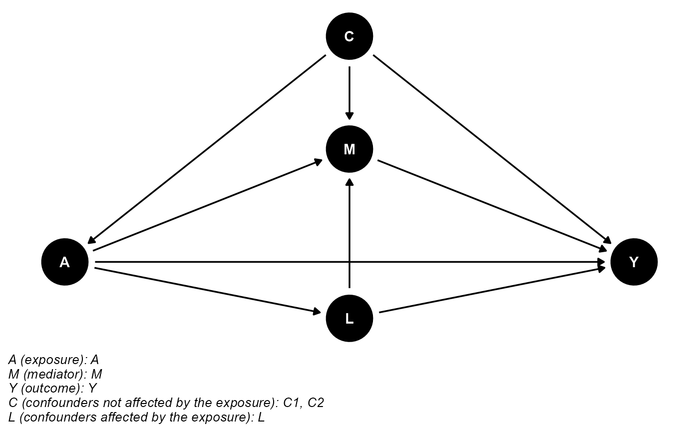
In this setting, we can use the marginal structural model and the -formula approach. The results are shown below.
The Marginal Structural Model
res_msm <- cmest(data = data, model = "msm", outcome = "Y", exposure = "A",
                 mediator = "M", basec = c("C1", "C2"), postc = "L", EMint = TRUE,
                 ereg = "logistic", yreg = "logistic", mreg = list("logistic"),
                 wmnomreg = list("logistic"), wmdenomreg = list("logistic"),
                 astar = 0, a = 1, mval = list(1),
                 estimation = "imputation", inference = "bootstrap", nboot = 2)
summary(res_msm)## Causal Mediation Analysis
##
## # Outcome regression:
##
## Call:
## glm(formula = Y ~ A + M + A * M, family = binomial(), data = getCall(x$reg.output$yreg)$data,
## weights = getCall(x$reg.output$yreg)$weights)
##
## Coefficients:
## Estimate Std. Error z value Pr(>|z|)
## (Intercept) -3.49700 0.47457 -7.369 1.72e-13 ***
## A 0.09466 0.67862 0.139 0.889
## M -0.40808 0.49218 -0.829 0.407
## A:M -0.79067 0.70198 -1.126 0.260
## ---
## Signif. codes: 0 '***' 0.001 '**' 0.01 '*' 0.05 '.' 0.1 ' ' 1
##
## (Dispersion parameter for binomial family taken to be 1)
##
## Null deviance: 1432.5 on 9999 degrees of freedom
## Residual deviance: 1412.9 on 9996 degrees of freedom
## AIC: 1432.5
##
## Number of Fisher Scoring iterations: 7
##
##
## # Mediator regressions:
##
## Call:
## glm(formula = M ~ A, family = binomial(), data = getCall(x$reg.output$mreg[[1L]])$data,
## weights = getCall(x$reg.output$mreg[[1L]])$weights)
##
## Coefficients:
## Estimate Std. Error z value Pr(>|z|)
## (Intercept) 2.96393 0.08185 36.211 < 2e-16 ***
## A 0.95266 0.11992 7.944 1.95e-15 ***
## ---
## Signif. codes: 0 '***' 0.001 '**' 0.01 '*' 0.05 '.' 0.1 ' ' 1
##
## (Dispersion parameter for binomial family taken to be 1)
##
## Null deviance: 2623.2 on 9999 degrees of freedom
## Residual deviance: 2560.6 on 9998 degrees of freedom
## AIC: 2580.5
##
## Number of Fisher Scoring iterations: 6
##
##
## # Mediator regressions for weighting (denominator):
##
## Call:
## glm(formula = M ~ A + C1 + C2 + L, family = binomial(), data = getCall(x$reg.output$wmdenomreg[[1L]])$data,
## weights = getCall(x$reg.output$wmdenomreg[[1L]])$weights)
##
## Coefficients:
## Estimate Std. Error z value Pr(>|z|)
## (Intercept) 0.9946 0.6067 1.639 0.1012
## A 1.8884 0.1726 10.944 < 2e-16 ***
## C1 1.4955 0.6090 2.456 0.0141 *
## C2 0.8166 0.1410 5.793 6.92e-09 ***
## L -0.9171 0.1215 -7.546 4.50e-14 ***
## ---
## Signif. codes: 0 '***' 0.001 '**' 0.01 '*' 0.05 '.' 0.1 ' ' 1
##
## (Dispersion parameter for binomial family taken to be 1)
##
## Null deviance: 2646.0 on 9999 degrees of freedom
## Residual deviance: 2397.3 on 9995 degrees of freedom
## AIC: 2407.3
##
## Number of Fisher Scoring iterations: 7
##
##
## # Mediator regressions for weighting (nominator):
##
## Call:
## glm(formula = M ~ A, family = binomial(), data = getCall(x$reg.output$wmnomreg[[1L]])$data,
## weights = getCall(x$reg.output$wmnomreg[[1L]])$weights)
##
## Coefficients:
## Estimate Std. Error z value Pr(>|z|)
## (Intercept) 2.93070 0.08064 36.345 <2e-16 ***
## A 0.99963 0.11952 8.364 <2e-16 ***
## ---
## Signif. codes: 0 '***' 0.001 '**' 0.01 '*' 0.05 '.' 0.1 ' ' 1
##
## (Dispersion parameter for binomial family taken to be 1)
##
## Null deviance: 2646.0 on 9999 degrees of freedom
## Residual deviance: 2576.3 on 9998 degrees of freedom
## AIC: 2580.3
##
## Number of Fisher Scoring iterations: 6
##
##
## # Exposure regression for weighting:
##
## Call:
## glm(formula = A ~ C1 + C2, family = binomial(), data = getCall(x$reg.output$ereg)$data,
## weights = getCall(x$reg.output$ereg)$weights)
##
## Coefficients:
## Estimate Std. Error z value Pr(>|z|)
## (Intercept) 0.08342 0.21440 0.389 0.69723
## C1 0.60899 0.21208 2.872 0.00409 **
## C2 0.10532 0.04375 2.407 0.01606 *
## ---
## Signif. codes: 0 '***' 0.001 '**' 0.01 '*' 0.05 '.' 0.1 ' ' 1
##
## (Dispersion parameter for binomial family taken to be 1)
##
## Null deviance: 12534 on 9999 degrees of freedom
## Residual deviance: 12520 on 9997 degrees of freedom
## AIC: 12526
##
## Number of Fisher Scoring iterations: 4
##
##
## # Effect decomposition on the odds ratio scale via the marginal structural model
##
## Direct counterfactual imputation estimation with
## bootstrap standard errors, percentile confidence intervals and p-values
##
## Estimate Std.error 95% CIL 95% CIU P.val
## Rcde 0.498566 0.044993 0.451404 0.512 <2e-16 ***
## rRpnde 0.539596 0.071146 0.460372 0.556 <2e-16 ***
## rRtnde 0.516788 0.055255 0.456013 0.530 <2e-16 ***
## rRpnie 0.986946 0.006183 0.994317 1.003 1
## rRtnie 0.945229 0.033333 0.948349 0.993 <2e-16 ***
## Rte 0.510041 0.052120 0.457210 0.527 <2e-16 ***
## ERcde -0.485135 0.050886 -0.546638 -0.478 <2e-16 ***
## rERintref 0.024731 0.020261 0.007245 0.034 <2e-16 ***
## rERintmed -0.016500 0.012843 -0.023146 -0.006 <2e-16 ***
## rERpnie -0.013054 0.006183 -0.005682 0.003 1
## ERcde(prop) 0.990156 0.003422 1.007348 1.012 <2e-16 ***
## rERintref(prop) -0.050476 0.044362 -0.073160 -0.014 <2e-16 ***
## rERintmed(prop) 0.033677 0.028384 0.010991 0.049 <2e-16 ***
## rERpnie(prop) 0.026643 0.012556 -0.004780 0.012 1
## rpm 0.060320 0.040940 0.006211 0.061 <2e-16 ***
## rint -0.016799 0.015978 -0.024035 -0.003 <2e-16 ***
## rpe 0.009844 0.003422 -0.011946 -0.007 <2e-16 ***
## ---
## Signif. codes: 0 '***' 0.001 '**' 0.01 '*' 0.05 '.' 0.1 ' ' 1
##
## (Rcde: controlled direct effect odds ratio; rRpnde: randomized analogue of pure natural direct effect odds ratio; rRtnde: randomized analogue of total natural direct effect odds ratio; rRpnie: randomized analogue of pure natural indirect effect odds ratio; rRtnie: randomized analogue of total natural indirect effect odds ratio; Rte: total effect odds ratio; ERcde: excess relative risk due to controlled direct effect; rERintref: randomized analogue of excess relative risk due to reference interaction; rERintmed: randomized analogue of excess relative risk due to mediated interaction; rERpnie: randomized analogue of excess relative risk due to pure natural indirect effect; ERcde(prop): proportion ERcde; rERintref(prop): proportion rERintref; rERintmed(prop): proportion rERintmed; rERpnie(prop): proportion rERpnie; rpm: randomized analogue of overall proportion mediated; rint: randomized analogue of overall proportion attributable to interaction; rpe: randomized analogue of overall proportion eliminated)
##
## Relevant variable values:
## $a
## [1] 1
##
## $astar
## [1] 0
##
## $yval
## [1] "1"
##
## $mval
## $mval[[1]]
## [1] 1The g-formula Approach
res_gformula <- cmest(data = data, model = "gformula", outcome = "Y", exposure = "A",
                      mediator = "M", basec = c("C1", "C2"), postc = "L", EMint = TRUE,
                      mreg = list("logistic"), yreg = "logistic", postcreg = list("linear"),
                      astar = 0, a = 1, mval = list(1),
                      estimation = "imputation", inference = "bootstrap", nboot = 2)
summary(res_gformula)## Causal Mediation Analysis
##
## # Outcome regression:
##
## Call:
## glm(formula = Y ~ A + M + A * M + C1 + C2 + L, family = binomial(),
## data = getCall(x$reg.output$yreg)$data, weights = getCall(x$reg.output$yreg)$weights)
##
## Coefficients:
## Estimate Std. Error z value Pr(>|z|)
## (Intercept) -2.7488 0.9365 -2.935 0.00333 **
## A -0.1267 0.6617 -0.192 0.84812
## M -0.7274 0.4136 -1.759 0.07863 .
## C1 -0.1906 0.8705 -0.219 0.82664
## C2 -0.5566 0.1933 -2.880 0.00397 **
## L -0.2242 0.1709 -1.312 0.18964
## A:M -0.3425 0.6635 -0.516 0.60572
## ---
## Signif. codes: 0 '***' 0.001 '**' 0.01 '*' 0.05 '.' 0.1 ' ' 1
##
## (Dispersion parameter for binomial family taken to be 1)
##
## Null deviance: 1447.7 on 9999 degrees of freedom
## Residual deviance: 1415.5 on 9993 degrees of freedom
## AIC: 1429.5
##
## Number of Fisher Scoring iterations: 7
##
##
## # Mediator regressions:
##
## Call:
## glm(formula = M ~ A + C1 + C2 + L, family = binomial(), data = getCall(x$reg.output$mreg[[1L]])$data,
## weights = getCall(x$reg.output$mreg[[1L]])$weights)
##
## Coefficients:
## Estimate Std. Error z value Pr(>|z|)
## (Intercept) 0.9946 0.6067 1.639 0.1012
## A 1.8884 0.1726 10.944 < 2e-16 ***
## C1 1.4955 0.6090 2.456 0.0141 *
## C2 0.8166 0.1410 5.793 6.92e-09 ***
## L -0.9171 0.1215 -7.546 4.50e-14 ***
## ---
## Signif. codes: 0 '***' 0.001 '**' 0.01 '*' 0.05 '.' 0.1 ' ' 1
##
## (Dispersion parameter for binomial family taken to be 1)
##
## Null deviance: 2646.0 on 9999 degrees of freedom
## Residual deviance: 2397.3 on 9995 degrees of freedom
## AIC: 2407.3
##
## Number of Fisher Scoring iterations: 7
##
##
## # Regressions for mediator-outcome confounders affected by the exposure:
##
## Call:
## glm(formula = L ~ A + C1 + C2, family = gaussian(), data = getCall(x$reg.output$postcreg[[1L]])$data,
## weights = getCall(x$reg.output$postcreg[[1L]])$weights)
##
## Coefficients:
## Estimate Std. Error t value Pr(>|t|)
## (Intercept) 1.00268 0.05077 19.75 <2e-16 ***
## A 1.00202 0.01081 92.68 <2e-16 ***
## C1 -1.00369 0.04980 -20.15 <2e-16 ***
## C2 -0.49437 0.01032 -47.92 <2e-16 ***
## ---
## Signif. codes: 0 '***' 0.001 '**' 0.01 '*' 0.05 '.' 0.1 ' ' 1
##
## (Dispersion parameter for gaussian family taken to be 0.2539334)
##
## Null deviance: 5324.2 on 9999 degrees of freedom
## Residual deviance: 2538.3 on 9996 degrees of freedom
## AIC: 14678
##
## Number of Fisher Scoring iterations: 2
##
##
## # Effect decomposition on the odds ratio scale via the g-formula approach
##
## Direct counterfactual imputation estimation with
## bootstrap standard errors, percentile confidence intervals and p-values
##
## Estimate Std.error 95% CIL 95% CIU P.val
## Rcde 0.499970 0.016697 0.638265 0.661 <2e-16 ***
## rRpnde 0.520367 0.029462 0.605367 0.645 <2e-16 ***
## rRtnde 0.507685 0.017636 0.627925 0.652 <2e-16 ***
## rRpnie 0.967499 0.024280 0.946213 0.979 <2e-16 ***
## rRtnie 0.943921 0.005571 0.981471 0.989 <2e-16 ***
## Rte 0.491185 0.032509 0.594150 0.638 <2e-16 ***
## ERcde -0.470168 0.008484 -0.330616 -0.319 <2e-16 ***
## rERintref -0.009465 0.020978 -0.063984 -0.036 <2e-16 ***
## rERintmed 0.003319 0.021233 0.014038 0.043 <2e-16 ***
## rERpnie -0.032501 0.024280 -0.053773 -0.021 <2e-16 ***
## ERcde(prop) 0.924046 0.049726 0.814903 0.882 <2e-16 ***
## rERintref(prop) 0.018602 0.043790 0.098667 0.157 <2e-16 ***
## rERintmed(prop) -0.006524 0.049233 -0.104694 -0.039 <2e-16 ***
## rERpnie(prop) 0.063876 0.055170 0.058171 0.132 <2e-16 ***
## rpm 0.057352 0.005937 0.019622 0.028 <2e-16 ***
## rint 0.012078 0.005444 0.052805 0.060 <2e-16 ***
## rpe 0.075954 0.049726 0.118289 0.185 <2e-16 ***
## ---
## Signif. codes: 0 '***' 0.001 '**' 0.01 '*' 0.05 '.' 0.1 ' ' 1
##
## (Rcde: controlled direct effect odds ratio; rRpnde: randomized analogue of pure natural direct effect odds ratio; rRtnde: randomized analogue of total natural direct effect odds ratio; rRpnie: randomized analogue of pure natural indirect effect odds ratio; rRtnie: randomized analogue of total natural indirect effect odds ratio; Rte: total effect odds ratio; ERcde: excess relative risk due to controlled direct effect; rERintref: randomized analogue of excess relative risk due to reference interaction; rERintmed: randomized analogue of excess relative risk due to mediated interaction; rERpnie: randomized analogue of excess relative risk due to pure natural indirect effect; ERcde(prop): proportion ERcde; rERintref(prop): proportion rERintref; rERintmed(prop): proportion rERintmed; rERpnie(prop): proportion rERpnie; rpm: randomized analogue of overall proportion mediated; rint: randomized analogue of overall proportion attributable to interaction; rpe: randomized analogue of overall proportion eliminated)
##
## Relevant variable values:
## $a
## [1] 1
##
## $astar
## [1] 0
##
## $yval
## [1] "1"
##
## $mval
## $mval[[1]]
## [1] 1